With a bit of trickery that is hard to spot, it is possible to “prove” that 1 + 1 = 3. (Watch this video and look carefully at the fourth and fifth lines of the “proof”, neither of which follows from the preceding line.)

Building on the logical and empirical analyses of some notable economists, I (and many others) have found the trickery in the “proof” that there is a fiscal multiplier: an additional dollar of government spending, not financed by borrowing or taxes) generates more than a dollar’s worth of additional GDP. The multiplier is both logically unsound and empirically invalid.

I urge you to read my page, “Keynesian Multiplier: Fiction vs. Fact“, for the details of my disproof. (For a recent discussion of the empirical invalidity of the multiplier, see this post by Veronique de Rugy.) I won’t repeat the details here, but I will focus on a particular aspect of the disproof. It exposes the logical trickery that underlies belief in the multiplier.

It used to be (and perhaps still is) the case that courses in the principles of macroeconomics began with a circular-flow model of a static economy. If everyone did the same thing, year after year, the same economic units would produce the same things. Each economic unit’s output would be valued in the marketplace, and that value would give the economic unit a claim on a slice of the total production of goods and services. The division of output between consumption (goods and services enjoyed here and now) and investment (replacement of the stock of capital as it deteriorates) would be determined by the willingness of producers (earners of income) to forgo consumption in favor of saving. (It is saving, non-consumption, that allows the diversion of resources to the production of capital goods.) The rate of investment would be just enough to sustain the output of goods and services at constant rates.

The circular flow could be perturbed for many reasons (e.g., population growth, a natural disaster, technological innovation). But what would happen to the circular flow in the event of such a perturbation? The output of goods and services would be increased or decreased by the immediate effect of the perturbation and by its secondary effects on the economy.

Take a simple two-producer economy, for example, where Joan makes guns and Ralph makes butter. Joan and Ralph exchange some of their output of guns and butter, so that during the year each of them earns a combination of guns and butter. If Ralph dies, and Joan is unable to make guns, the only output will be butter. And if Joan doesn’t need as much butter as she used to produce (some of which she traded to Ralph for guns), she will produce less butter — just enough for her own consumption. So there is the immediate effect of Ralph’s death (no guns) and the secondary effect of Ralph’s death (Joan produces less butter but consumes the same amount as before).

The multiplier doesn’t work that way. According to the multiplier, the reduction in Ralph’s spending on butter would affect Joan’s spending according to her marginal propensity to consume (the rate at which each increment of her income is translated into more or less spending on consumption goods). But it doesn’t. Joan, quite sensibly, simply consumes as much butter as before, though she produces less of it. There is no multiplier effect. There is just a reduction in the economy’s total output: no guns, and just enough butter for Joan’s needs.

A defender of the multiplier would respond that my economy doesn’t represent an advanced economy like that of the United States, in which most transactions don’t take place at arms length (through barter) but, rather, through a medium of exchange (U.S. dollars). In such an economy, the defenders would argue, an exogenous reduction or increase in the demand for goods and services would cascade through the economy. Less demand for A would reduce the income of the producer of A, who would spend less on B through Z; the producer of B would spend less on A and C through Z; etc. In the end, the economy would shrink by the sum of each producer’s reduced spending — the multiplier effect. Here is the standard derivation of that effect, which I explain here:

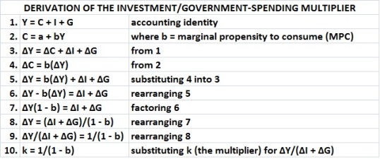
Y is GDP, C is consumption spending, I is investment spending, G is government spending (all in “real” terms), and b (as stated) is the marginal propensity to consume.)

Because b is less than 1, the expression 1/(1-b) must be greater than 1 — thus the “multiplier” on an exogenous change in spending. And despite the heading, the multiplier effect, in theory, applies to any exogenous change in the amount or rate of spending or saving. It could be a consumption or saving multiplier, for example. That is one of the tricks of the multiplier: If it exists, it isn’t just a government-spending multiplier, much as the proponents of bigger government would like you to believe.

Another trick is the mysterious mechanism by which an exogenous change in the rate of spending results in even more spending. It’s time to expose the mechanism.

What is Y but the sum of the dollar values (adjusted for inflation) of the output of all “final” goods and services (including changes in inventory) during a given period? What does Y therefore represent? As long as we’re using the terminology of macroeconomics, in which everything is implicitly homogeneous, Y represents the familiar (to some) equation of exchange:

MV = PQ, where, for a given period,

M is the total nominal amount of money supply in circulation on average in an economy.

V is the velocity of money, that is the average frequency with which a unit of money is spent.

P is the price level.

Q is an index of real expenditures (on newly produced goods and services).

The multiplier implies that, everything else being the same, a change in Q will result in proportional changes in PQ and MV. If there are unemployed resources and an exogenous increase in government spending employs them (and does nothing to prices), an increase in M (deficit spending) is exactly matched by an increase in Q (real output), so that the equation MV = PQ isn’t violated.

But how does an increase in Q (the initial burst of additional output) result in further additions to Q, as the multiplier implies? If P doesn’t increase (and it shouldn’t if the multiplier is “real”), then MV must rise. There is an increase in M — the jolt of exogenous government spending. But there is no further increase in M. So MV must rise because V increases as a result of the initial jolt of government spending. The multiplier, however, says nothing about V, unless increases in spending that result from the initial jolt in Q can be construed as increases in V and Q.

Let’s step back from this conundrum and consider the situation of a static economy with unemployed resources. An increase in M (deficit spending), of targeted perfectly, resulting in a proportional increase in Q. The persons who earn income from that increase spend some of it (that is, their rate of spending rises temporarily). There is no new M, but V rises (that is, the rate of spending rises) in proportion to the rise Q. So, temporarily, MV’ = PQ’.

This is the only sensible way of explaining the multiplier. But look at how many things must happen if an exogenous increase in government spending is to result in an actual increase real output:

The additional spending must be targeted so that it elicits additional production from unemployed resources.

The addition production must, somehow, be delivered to persons who actually benefit from it.

The recipients of additional spending must at least some of their new income into spending that results in the employment of hitherto unemployed resources, and the result must be the production of additional things that are delivered to persons who benefit from the production.

And so on and so forth.

What happens in practice, of course, is that deficit spending results in the production of things that politicians and bureaucrats favor (e.g., economically useless bullet trains and bridges to nowhere). but which have little or no economic value. And the spending often crowds out the production of other things because many (most?) of the resources involved are already in use (e.g., engineers and trained mechanics, not unemployed high-school dropouts from inner cities). Those are among that many things that are skipped over in the “proof” that the multiplier is real and positive. (See my page about the multiplier for much more.)

The bottom line is that the multiplier might well be positive, in nominal terms. That is, GDP might seem to rise, at least temporarily, but real GDP — the actual output of things valued by consumers — is another matter entirely. As I suggest here — and as is pointed out in my page about the multiplier and the article by Veronique de Rugy — the actual output of things valued by consumers may not rise at all, and probably will be crowded out by additional government spending.

Things valued by consumers certainly will be crowded out by additional government spending, because — in the long run — temporary additions usually become permanent ones. Which is just what the proponents of the multiplier want to happen. The multiplier isn’t just phony, it’s an excuse to boost government spending, that is, the share of the economy that is directly controlled by government.

Have you noticed lately what a great job government is doing for the citizenry, especially in Blue States and cities?