REVISED 02/09/15 WITH AN ADDENDUM AT THE END OF THE POST
This post is prompted by a reader’s comments about “The Compleat Monty Hall Problem.” I open with a discussion of probability and its inapplicability to single games of chance (e.g., one toss of a coin). With that as background, I then address the reader’s specific comments. I close with a discussion of the debasement of the meaning of probability.
INTRODUCTORY REMARKS
What is probability? Is it a property of a thing (e.g., a coin), a property of an event involving a thing (e.g., a toss of the coin), or a description of the average outcome of a large number of such events (e.g., “heads” and “tails” will come up about the same number of times)? I take the third view.
What does it mean to say, for example, that there’s a probability of 0.5 (50 percent) that a tossed coin will come up “heads” (H), and a probability of 0.5 that it will come up “tails” (T)? Does such a statement have any bearing on the outcome of a single toss of a coin? No, it doesn’t. The statement is only a short way of saying that in a sufficiently large number of tosses, approximately half will come up H and half will come up T. The result of each toss, however, is a random event — it has no probability.
That is the standard, frequentist interpretation of probability, to which I subscribe. It replaced the classical interpretation , which is problematic:
If a random experiment can result in N mutually exclusive and equally likely outcomes and if NA of these outcomes result in the occurrence of the event A, the probability of A is defined by
 .
.
There are two clear limitations to the classical definition.[16] Firstly, it is applicable only to situations in which there is only a ‘finite’ number of possible outcomes. But some important random experiments, such as tossing a coin until it rises heads, give rise to an infinite set of outcomes. And secondly, you need to determine in advance that all the possible outcomes are equally likely without relying on the notion of probability to avoid circularity….
A similar charge has been laid against frequentism:
It is of course impossible to actually perform an infinity of repetitions of a random experiment to determine the probability of an event. But if only a finite number of repetitions of the process are performed, different relative frequencies will appear in different series of trials. If these relative frequencies are to define the probability, the probability will be slightly different every time it is measured. But the real probability should be the same every time. If we acknowledge the fact that we only can measure a probability with some error of measurement attached, we still get into problems as the error of measurement can only be expressed as a probability, the very concept we are trying to define. This renders even the frequency definition circular.
Not so:
- There is no “real probability.” If there were, the classical theory would measure it, but the classical theory is circular, as explained above.
- It is therefore meaningless to refer to “error of measurement.” Estimates of probability may well vary from one series of trials to another. But they will “tend to a fixed limit” over many trials (see below).
There are other approaches to probability. See, for example, this, this, and this.) One approach is known as propensity probability:
Propensities are not relative frequencies, but purported causes of the observed stable relative frequencies. Propensities are invoked to explain why repeating a certain kind of experiment will generate a given outcome type at a persistent rate. A central aspect of this explanation is the law of large numbers. This law, which is a consequence of the axioms of probability, says that if (for example) a coin is tossed repeatedly many times, in such a way that its probability of landing heads is the same on each toss, and the outcomes are probabilistically independent, then the relative frequency of heads will (with high probability) be close to the probability of heads on each single toss. This law suggests that stable long-run frequencies are a manifestation of invariant single-case probabilities.
This is circular. You observe the relative frequencies of outcomes and, lo and behold, you have found the “propensity” that yields those relative frequencies.
Another approach is Bayesian probability:
Bayesian probability represents a level of certainty relating to a potential outcome or idea. This is in contrast to a frequentist probability that represents the frequency with which a particular outcome will occur over any number of trials.
An event with Bayesian probability of .6 (or 60%) should be interpreted as stating “With confidence 60%, this event contains the true outcome”, whereas a frequentist interpretation would view it as stating “Over 100 trials, we should observe event X approximately 60 times.”
Or consider this account:
The Bayesian approach to learning is based on the subjective interpretation of probability. The value of the proportion p is unknown, and a person expresses his or her opinion about the uncertainty in the proportion by means of a probability distribution placed on a set of possible values of p….
“Level of certainty” and “subjective interpretation” mean “guess.” The guess may be “educated.” It’s well known, for example, that a balanced coin will come up heads about half the time, in the long run. But to say that “I’m 50-percent confident that the coin will come up heads” is to say nothing meaningful about the outcome of a single coin toss. There are as many probable outcomes of a coin toss as there are bystanders who are willing to make a statement like “I’m x-percent confident that the coin will come up heads.” Which means that a single toss doesn’t have a probability, though it can be the subject of many opinions as to the outcome.
Returning to reality, Richard von Mises eloquently explains frequentism in Probability, Statistics and Truth (second revised English edition, 1957). Here are some excerpts:
The rational concept of probability, which is the only basis of probability calculus, applies only to problems in which either the same event repeats itself again and again, or a great number of uniform elements are involved at the same time. Using the language of physics, we may say that in order to apply the theory of probability we must have a practically unlimited sequence of uniform observations. [P. 11]
* * *
In games of dice, the individual event is a single throw of the dice from the box and the attribute is the observation of the number of points shown by the dice. In the game of “heads or tails”, each toss of the coin is an individual event, and the side of the coin which is uppermost is the attribute. [P. 11]
* * *
We must now introduce a new term…. This term is “the collective”, and it denotes a sequence of uniform events or processes which differ by certain observable attributes…. All the throws of dice made in the course of a game [of many throws] from a collective wherein the attribute of the single event is the number of points thrown…. The definition of probability which we shall give is concerned with ‘the probability of encountering a single attribute in a given collective’. [Pp. 11-12]
* * *
[A] collective is a mass phenomenon or a repetitive event, or, simply, a long sequence of observations for which there are sufficient reasons to believe that the relative frequency of the observed attribute would tend to a fixed limit if the observations were indefinitely continued. The limit will be called the probability of the attribute considered within the collective. [P. 15, emphasis in the original]
* * *
The result of each calculation … is always … nothing else but a probability, or, using our general definition, the relative frequency of a certain event in a sufficiently long (theoretically, infinitely long) sequence of observations. The theory of probability can never lead to a definite statement concerning a single event. The only question that it can answer is: what is to be expected in the course of a very long sequence of observations? [P. 33, emphasis added]
As stated earlier, it is simply meaningless to say that the probability of H or T coming up in a single toss is 0.5. Here’s the proper way of putting it: There is no reason to expect a single coin toss to have a particular outcome (H or T), given that the coin is balanced, the toss isn’t made is such a way as to favor H or T, and there are no other factors that might push the outcome toward H or T. But to say that P(H) is 0.5 for a single toss is to misrepresent the meaning of probability, and to assert something meaningless about a single toss.
If you believe that probabilities attach to a single event, you must also believe that a single event has an expected value. Let’s say, for example, that you’re invited to toss a coin once, for money. You get $1 if H comes up; you pay $1 if T comes up. As a believer in single-event probabilities, you “know” that you have a “50-50 chance” of winning or losing. Would you play a single game, which has an expected value of $0? If you would, it wouldn’t be because of the expected value of the game; it would be because you might win $1, and because losing $1 would mean little to you.
Now, change the bet from $1 to $1,000. The “expected value” of the single game remains the same: $0. But the size of the stake wonderfully concentrates your mind. You suddenly see through the “expected value” of the game. You are struck by the unavoidable fact that what really matters is the prospect of winning $1,000 or losing $1,000, because those are the only possible outcomes.
Your decision about playing a single game for $1,000 will depend on your finances (e.g., you may be very wealthy or very desperate for money) and your tolerance for risk (e.g., you may be averse to risk-taking or addicted to it). But — if you are rational — you will not make your decision on the basis of the fictional expected value of a single game, which derives from the fictional single-game probabilities of H and T. You will decide whether you’re willing and able to risk the loss of $1,000.
Do I mean to say that probability is irrelevant to a single play of the Monty Hall problem, or to a choice between games of chance? If you’re a proponent of propensity, you might say that in the Monty Hall game the prize has a propensity to be behind the other unopened door (i.e., the door not chosen by you and not opened by the host). But does that tell you anything about the actual location of the prize in a particular game? No, because the “propensity” merely reflects the outcomes of many games; it says nothing about a single game, which (like Schrödinger’s cat) can have only a single outcome (prize or no prize), not 2/3 of one.
If you’re a proponent of Bayesian probability, you might say that you’re confident with “probability” 2/3 that the prize is behind the other unopened door. But that’s just another way of saying that contestants win 2/3 of the time if they always switch doors. That’s the background knowledge that you bring to your statement of confidence. But someone who’s ignorant of the Monty Hall problem might be confident with 1/2 “probability” that the prize is behind the other unopened door. And he could be right about a particular game, despite his lower level of confidence.
So, yes, I do mean to say that there’s no such thing as a single-case probability. You may have an opinion ( or a hunch or a guess) about the outcome of a single game, but it’s only your opinion (hunch, guess). In the end, you have to bet on a discrete outcome. If it gives you comfort to switch to the unopened door because that’s the winning door 2/3 of the time (according to classical probability) and about 2/3 of the time (according to the frequentist interpretation), be my guest. I might do the same thing, for the same reason: to be comfortable about my guess. But I’d be able separate my psychological need for comfort from the reality of the situation:
A single game is just one event in the long series of events from which probabilities emerge. I can win the Monty Hall game about 2/3 of the time in repeated plays if I always switch doors. But that probability has nothing to do with a single game, the outcome of which is a random occurrence.
REPLIES TO A READER’S COMMENTS
I now turn to the reader’s specific comments, which refer to “The Compleat Monty Hall Problem.” (You should read it before continuing with this post if you’re unfamiliar with the Monty Hall problem or my analysis of it.) The reader’s comments — which I’ve rearranged slightly — are in italic type. (Here and there, I’ve elaborated on the reader’s comments; my elaborations are placed in brackets and set in roman type.) My replies are in bold type.
I find puzzling your statement that a probability cannot “describe” a single instance, eg one round of the Monty Hall problem.
See my introductory remarks.
While the long run result serves to prove the probability of a particular outcome, that does not mean that that probability may not be assigned to a smaller number of instances. That is the beauty of probability.
The long-run result doesn’t “prove” the probability of a particular outcome; it determines the relative frequency of occurrence of that outcome — and nothing more. There is no probability associated with a “smaller number of instances,” certainly not 1 instance. Again, see my introductory remarks.
If the [Monty Hall] game is played once [and I don’t switch doors], I should budget for one car [the prize that’s usually cited in discussions of the Monty hall problem], and if it is played 100 times [and I never switch doors], I budget for 33….
“Budget” seems to refer to the expected number of cars won, given the number of plays of the game and a strategy of never switching doors. The reader contradicts himself by “budgeting” for 1 car in a single play of the Monty Hall problem. In doing so, he is being unfaithful to his earlier statement: “While the long run result serves to prove the probability of a particular outcome, that does not mean that that probability may not be assigned to a smaller number of instances.” Removing the double negatives, we get “probability may be assigned to a smaller number of instances.” Given that 1 is a smaller number than 100, it follows, by the reader’s logic, that his “budget” for a single game should be 1/3 car (assuming, as he does, a strategy of not switching doors). The reader’s problem here is his insistence that a probability expresses something other than the long-run relative frequency of a particular outcome.
To justify your contrary view, you ask how you can win 2/3 of a car [the long-run average if the contestant plays many games and always switches doors]; you can win or you can not win, you say, you cannot partly win. Is this not sophistry or a straw man, sloppy reasoning at best, to convince uncritical thinkers who agree that you cannot drive 2/3 of a car?
My “contrary view” of what? My view of statistics isn’t “contrary.” Rather, it’s in line with the standard, frequentist interpretation.
It’s a simple statement of obvious fact you can’t win 2/3 of a car. There’s no “sophistry” or “straw man” about it. If you can’t win 2/3 of a car, what does it mean to assign a probability of 2/3 to winning a car by adopting the switching strategy? As discussed above, it means only one thing: A long series of games will be won about 2/3 of the time if all contestants adopt the switching strategy.
On what basis other than an understanding of probability would you be optimistic at the prospect of being offered one chance of picking a single Golden Ball worth $1m from a bag of just three balls and pessimistic about your prospects of picking the sole Golden Ball from a barrel of 10,000 balls?
The only difference between the two games is that on the one hand you have a decent (33%) chance of winning and on the other hand you have a lousy (0.01%) chance. Isn’t it these disparate probabilities that give you cause for optimism or pessimism, as the case may be?
“Optimism” and “pessimism” — like “comfort” — are subjective terms for ill-defined states of mind. There are persons who will be “optimistic” about a given situation, and persons who will be “pessimistic” about the same situation. For example: There are hundreds of millions of persons who are “optimistic” about winning various lotteries, even though they know that the grand prize in each lottery will be assigned to only one of millions of possible numbers. By the same token, there are hundreds of millions of persons who, knowing the same facts, refuse to buy lottery tickets because they are “pessimistic” about the likely outcome of doing so. But “optimism” and “pessimism” — like “comfort” — have nothing to do with probability, which isn’t an attribute of a single game.
If probability cannot describe the chances of each of the two one-off “games”, does that mean I could not provide a mathematical basis for my advice that you play the game with 3 balls (because you have a one-in-three chance of winning) rather than the ball in the barrel game which offers a one in ten thousand chance of winning?
You can provide a mathematical basis for preferring the game with 3 balls. But you must, in honesty, state that the mathematical basis applies only to many games, and that the outcome of a single game is unpredictable.
It might be that probability cannot reliably describe the actual outcome of a single event because the sample size of 1 game is too small to reflect the long-run average that proves the probability. However, comparing the probabilities for winning the two games describes the relative likelihood of winning each game and informs us as to which game will more likely provide the prize.
If not by comparing the probability of winning each game, how do we know which of the two games has a better chance of delivering a win? One cannot compare the probability of selecting the Golden Ball from each of the two games unless the probability of each game can be expressed, or described, as you say.
Here, the reader comes close to admitting that a probability can’t describe the (expected) outcome of a single event (“reliably” is superfluous). But he goes off course when he says that “comparing the probabilities for the two games … informs us as to which game will more likely provide the prize.” That statement is true only for many plays of the two ball games. It has nothing to do with a single play of either ball game. The choice there must be based on subjective considerations: “optimism,” “pessimism,” “comfort,” a guess, a hunch, etc.
Can I not tell a smoker that their lifetime risk of developing lung cancer is 23% even though smokers either get lung cancer or they do not? No one gets 23% cancer. Did someone say they did? No one has 0.2 of a child either but, on average, every family in a census did at one stage have 2.2 children.
No, the reader may not (honestly) tell a smoker that his lifetime risk of developing lung cancer is 23 percent, or any specific percentage. The smoker has one life to live; he will either get lung cancer or he will not. What the reader may honestly tell the smoker is that statistics based on the fates of a large number of smokers over many decades indicate that a certain percentage of those smokers contracted lung cancer. The reader should also tell the smoker that the frequency of the incidence of lung cancer in a large population varies according to the number of cigarettes smoked daily. (According to Wikipedia: “For every 3–4 million cigarettes smoked, one lung cancer death occurs.[1][132]“) Further, the reader should note that the incidence of lung cancer also varies with the duration of smoking at various rates, and with genetic and environmental factors that vary from person to person.
As for family size, given that the census counts only post-natal children (who come in integer values), how could “every family in a census … at one stage have 2.2 children”? The average number of children across a large number of families may be 2.2, but surely the reader knows that “every family” did not somehow have 2.2 children “at one stage.” And surely the reader knows that average family size isn’t a probabilistic value, one that measures the relative frequency of an event (e.g., “heads”) given many repetitions of the same trial (e.g., tossing a fair coin), under the same conditions (e.g., no wind blowing). Each event is a random occurrence within the long string of repetitions. The reader may have noticed that family size is in fact strongly determined (especially in Western countries) by non-random events (e.g., deliberate decisions by couples to reproduce, or not). In sum, probabilities may represent averages, but not all (or very many) averages represent probabilities.
If not [by comparing probabilities], how do we make a rational recommendation and justify it in terms the board of a think-tank would accept? [This seems to be a reference to my erstwhile position as an officer of a defense think-tank.]
Here, the reader extends an inappropriate single-event view of probability to an inappropriate unique-event view. I would not have gone before the board and recommended a course of action — such as bidding on a contract for a new line of work — based on a “probability of success.” That would be an absurd statement to make about an event that is defined by unique circumstances (e.g., the composition of the think-tank’s staff at that time, the particular kind of work to be done, the qualifications of prospective competitors’ staffs). I would simply have spelled out the facts and the uncertainties. And if I had a hunch about the likely success or failure of the venture, I would have recommended for or against it, giving specific reasons for my hunch (e.g., the relative expertise of our staff and competitors’ staffs). But it would have been nothing more than a hunch; it wouldn’t have been my (impossible) assessment of the probability of a unique event.
Boards (and executives) don’t base decisions on (non-existent) probabilities; they base decisions on unique sets of facts, and on hunches (preferably hunches rooted in knowledge and experience). Those hunches may sometimes be stated as probabilities, as in “We’ve got a 50-50 chance of winning the contract.” (Though I would never say such a thing.) But such statements are only idiomatic, and have nothing to do with probability as it is properly understood.
CLOSING THOUGHTS
The reader’s comments reflect the popular debasement of the meaning of probability. The word has been adapted to many inappropriate uses: the probability of precipitation (a quasi-subjective concept), the probability of success in a business venture (a concept that requires the repetition of unrepeatable events), the probability that a batter will get a hit in his next at-bat (ditto, given the many unique conditions that attend every at-bat), and on and on. The effect of all such uses (and, often, the purpose of such uses) is to make a guess seem like a “scientific” prediction.
ADDENDUM (02/09/15)
The reader whose comments about “The Compleat Monty Hall Problem” I address above has submitted some additional comments.
The first additional comment pertains to this exchange where the reader’s remarks are in italics and my reply is in bold:
If the [Monty Hall] game is played once [and I don’t switch doors], I should budget for one car [the prize that’s usually cited in discussions of the Monty hall problem], and if it is played 100 times [and I never switch doors], I budget for 33….
“Budget” seems to refer to the expected number of cars won, given the number of plays of the game and a strategy of never switching doors. The reader contradicts himself by “budgeting” for 1 car in a single play of the Monty Hall problem. In doing so, he is being unfaithful to his earlier statement: “While the long run result serves to prove the probability of a particular outcome, that does not mean that that probability may not be assigned to a smaller number of instances.” Removing the double negatives, we get “probability may be assigned to a smaller number of instances.” Given that 1 is a smaller number than 100, it follows, by the reader’s logic, that his “budget” for a single game should be 1/3 car (assuming, as he does, a strategy of not switching doors). The reader’s problem here is his insistence that a probability expresses something other than the long-run relative frequency of a particular outcome.
The reader’s rejoinder (with light editing by me):
The game-show producer “budgets” one car if playing just one game because losing one car is a possible outcome and a prudent game-show producer would cover all possibilities, the loss of one car being one of them. This does not contradict anything I have said, it is simply the necessary approach to manage the risk of having a winning contestant and no car. Similarly, the producer budgets 33 cars for a 100-show season [TEA: For consistency, “show” should be “game”].
The contradiction is between the reader’s use of an expected-value calculation for 100 games, but not for a single game. If the game-show producer knows (how?) that contestants will invariably stay with the doors they’ve chosen initially, a reasonable budget for a 100-game season is 33 cars. (But a “reasonable” budget isn’t a foolproof one, as I show below.) By the same token, a reasonable budget for a single game — a game played only once, not one game in a series — is 1/3 car. After all, that is the probabilistic outcome of a single game if you believe that a probability can be assigned to a single game. And the reader does believe that; here’s the first sentence of his original comments:
I find puzzling your statement that a probability cannot “describe” a single instance, eg one round of the Monty Hall problem. [See the section “Replies to a Reader’s Comments” in “Some Thoughts about Probability.”]
Thus, according the reader’s view of probability, the game-show producer should budget for 1/3 car. After all, in the reader’s view, there’s a 2/3 probability that a contestant won’t win a car in a one-game run of the show.
The reader could respond that cars come in units of one. True, but the designation of a car as the prize is arbitrary (and convenient for the reader). The prize could just as well be money — $30,000 for example. If the contestant wins a car in the (rather contrived) one-game run of the show, the producer then (and only then) gives the contestant a check for $30,000. But, by the reader’s logic, the game has two other equally likely outcomes: the contestant loses and the contestant loses. If those outcomes prevail, the producer doesn’t have to write a check. So, the average prize for the one-game run of the show would be $10,000, or the equivalent of 1/3 car.
Now, the producer might hedge his bets because the outcome of a single game is uncertain; that is, he might budget one car or $30,000. But by the same logic, the producer should budget 100 cars or $3,000,000 for 100 games, not 33 cars or $990,000. Again, the reader contradicts himself. He uses an expected-value calculation for one game but not for 100 games.
What is a “reasonable” budget for 100 games, or fewer than 100 games? Well, it’s really a subjective call that the producer must make, based on his tolerance for risk. The producer who budgets 33 cars or $990,000 for 100 games on the basis of an expected-value calculation may find himself without a job.
Using a random-number generator, I set up a simulation of the outcomes of games 1 through 100, where the contestant always stays with the door originally chosen . Here are the results of the first five simulations that I ran:
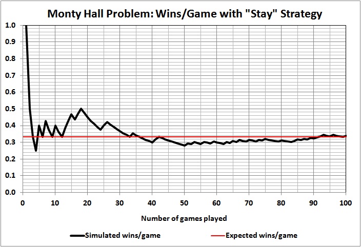
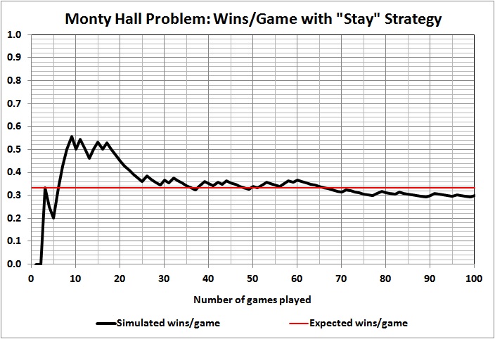
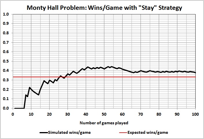
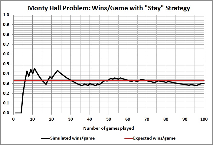
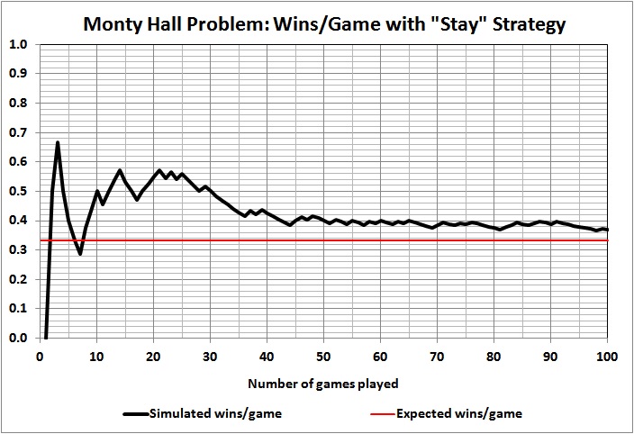
Some observations:
Outcomes of individual games are unpredictable, as evidenced by the wild swings and jagged lines, the latter of which persist even at 100 games.
Taking the first game as a proxy for a single-game run of the show, we see that the contestant won that game in just one of the five simulations. To put it another way, in four of the five cases the producer would have thrown away his money on a rapidly depreciating asset (a car) if had offered a car as the prize.
Results vary widely and wildly after the first game. At 10 and 20 games, contestants are doing better than expected in four of the five simulations. At 30 games, contestants are doing as well or better than expected in all five simulations. At 100 games, contestants are doing better than expected in two simulation, worse than expected in two simulation, and exactly as expected in one simulation. What should the producer do with such information? Well, it’s up to the producer and his tolerance for risk. But a prudent producer wouldn’t budget 33 cars or $990,000 just because that’s the expected value of 100 games.
It can take a lot of games to yield an outcome that comes close to 1/3 car per game. A game-show producer could easily lose his shirt by “betting” on 1/3 car per game for a season much shorter than 100 games, and even for a season of 100 games.
* * *
The reader’s second additional comment pertains to this exchange:
On what basis other than an understanding of probability would you be optimistic at the prospect of being offered one chance of picking a single Golden Ball worth $1m from a bag of just three balls and pessimistic about your prospects of picking the sole Golden Ball from a barrel of 10,000 balls?
The only difference between the two games is that on the one hand you have a decent (33%) chance of winning and on the other hand you have a lousy (0.01%) chance. Isn’t it these disparate probabilities that give you cause for optimism or pessimism, as the case may be?
“Optimism” and “pessimism” — like “comfort” — are subjective terms for ill-defined states of mind. There are persons who will be “optimistic” about a given situation, and persons who will be “pessimistic” about the same situation. For example: There are hundreds of millions of persons who are “optimistic” about winning various lotteries, even though they know that the grand prize in each lottery will be assigned to only one of millions of possible numbers. By the same token, there are hundreds of millions of persons who, knowing the same facts, refuse to buy lottery tickets because they are “pessimistic” about the likely outcome of doing so. But “optimism” and “pessimism” — like “comfort” — have nothing to do with probability, which isn’t an attribute of a single game.
The reader now says this:
Optimism or pessimism are states as much as something being hot or cold, or a person perspiring or not, and one would find a lot more confidence among contestants playing a single instance of a 1-in-3 game than one would find amongst contestants playing a 1-in-1b game.
Apart from differing probabilities, how would you explain the higher levels of confidence among players of the 1-in-3 game?
Alternatively, what about a “game” involving 2 electrical wires, one live and one neutral, and a game involving one billion electrical wires, only one of which is live? Contestants are offered $1m if they are prepared to touch one wire. No one accepts the dare in the 1-in-2 game but a reasonable percentage accept the dare in the 1-in-1b game.
Is the probable outcome of a single event a factor in the different rates of uptake between the two games?
The reader begs the question by introducing “hot or cold” and “perspiring or not,” which have nothing to do with objective probabilities (long-run frequencies of occurrence) and everything to do with individual attitudes toward risk-taking. That was the point of my original response, and I stand by it. The reader simply tries to evade the point by reading the minds of his hypothetical contestants (“higher levels of confidence among players of the 1-in-3 game”). He fails to address the basic issue, which is whether or not there are single-case probabilities — an issue that I addressed at length in “Some Thoughts…”.
The alternative hypotheticals involving electrical wires are just variants of the original one. They add nothing to the discussion.
* * *
Enough of this. If the reader — or anyone else — has some good arguments to make in favor of single-case probabilities, drop me a line. If your thoughts have merit, I may write about them.