GDP Update

Posted on November 26, 2020 by Loquitur Veritatem

The Bureau of Economic Analysis yesterday released its revised (second) estimate of GDP for the third quarter of 2020 (2020Q3). The recovery from the recession that was induced by COVID-19 lockdown orders continues, but there’s still a lot of lost ground to make up. And the lost ground to be made up isn’t just from the pre-COVID-19 rate of output, but from the post-Great Recession slump that persisted despite Trump’s deregulatory efforts.

Here’s the big picture:

This graph zooms in on the declining rate of growth in real GDP:

This graph highlights the declining rate of growth from business cycle to business cycle:

The unnecessarily draconian response to COVID-19 made a bad situation even worse.

The Economic Damage of COVID-19: A Preliminary Assessment

Posted on April 29, 2020 by Loquitur Veritatem

The Bureau of Economic Analysis today released its advance (first) estimate of GDP for the first quarter of 2020, which is now almost a month in the past. The year-over-year change in real GDP was 0.3 percent (a slight increase). The annualized decline in quarterly GDP was 4.8 percent, the worst since the 8.4 percent decline in the fourth quarter of 2008 (the year of the financial meltdown).

Here’s how the first quarter of 2020 looks in the context of post-World War II changes in GDP:

If, as I expect, the incipient COVID-19 recession of 2020 ends quickly (perhaps in the third or fourth quarter of the year), it will prove to be less damaging (economically) than previous post-war recessions. That won’t be of solace to those who have suffered through the disease, lost loved ones, lost their jobs and businesses, and seen their investments decline in value.

But (economically) it is better than the alternative, which is something on the order of the Great Recession or Great Depression. The former spanned 3-1/2 years, from the time of its onset until real GDP finally rose above the pre-recession level. The latter spanned 1929-1936, was followed by a recession in 1937-1938, and didn’t end decisively until after World War II.

GDP Trivia

Posted on October 30, 2019 by Loquitur Veritatem

Bearing in mind Arnold Kling’s reservations (and my own) about aggregate economic data, I will nevertheless entertain you with some trivial factoids on the occasion of the release of the 3rd quarter 2019 GDP estimate (advance estimate).

First, the post-World War II business-cycle record:

Graphically (with short cycles omitted):

The current cycle is the second-longest since the end of World War II, but also the least robust.

Note the large gap between the (low) peak growth rates experienced in recent cycles (purple, pale green, and red lines) and the (higher ones) experienced in earlier cycles. The peak for the current cycle (if you can call it a peak) occurred early (in the 5th quarter after the bottom of the Great Recession). Such a low peak so early in the cycle broke a pattern that had held since the end of World War II:

The red diamond represents the current cycle. Earlier cycles are represented by black dots, and the robust regression equation applies to those cycles.

I won’t be surprised if economists discover that the weakness of the current business cycle is due to Obama’s economic policies (and rhetoric), just as economists (unsurprisingly) discovered that FDR’s policies deepened and prolonged the Great Depression.

Unorthodox Economics: 5. Economic Progress, Microeconomics, and Microeconomics

Posted on July 13, 2018 by Loquitur Veritatem

This is the fifth entry in what I hope will become a book-length series of posts. That result, if it comes to pass, will amount to an unorthodox economics textbook. Here are the chapters that have been posted to date:

1. What Is Economics?
2. Pitfalls
3. What Is Scientific about Economics?
4. A Parable of Political Economy
5. Economic Progress, Microeconomics, and Macroeconomics

What is economic progress? It is usually measured as an increase in gross domestic product (GDP) or, better yet, per-capita GDP. But such measures say nothing about the economic status or progress of particular economic units. In fact, the economic progress of some economic units will be accompanied by the economic regress of others. GDP captures the net monetary effect of those gains and losses. And if the net effect is positive, the nation under study is said to have made economic progress. But that puts the cart of aggregate measures (macroeconomics) before the horse of underlying activity (microeconomics). This chapter puts them in the right order.

The economy of the United States (or any large political entity) consists of myriad interacting units. Some of them contribute to the output of the economy; some of them constrain the output; some of them are a drain upon it. The contributing units are the persons, families, private charities, and business (small and large) that produce economic goods (products and services) which are voluntarily exchanged for the mutual benefit of the trading parties. (Voluntary, private charities are among the contributing units because they help willing donors attain the satisfaction of improving the lot of persons in need. Voluntary charity — there is no other kind — is not a drain on the economy.)

Government is also a contributing unit to the extent that it provides a safe zone for the production and exchange of economic goods, to eliminate or reduce the debilitating effects of force and fraud. The safe zone is international as well as domestic when the principals of the U.S. government have the wherewithal and will to protect Americans’ overseas interests. The provision of a safe zone is usually referred to as the “rule of law”.

Most other governmental functions constrain or drain the economy. Those functions consist mainly of regulatory hindrances and forced “charity,” which includes Social Security, Medicare, Medicaid, and other federal, State, and local “welfare” programs. In “The Rahn Curve Revisited,” I estimate the significant negative effects of regulation and government spending on GDP.

There is a view that government contributes directly to economic progress by providing “infrastructure” (e.g., the interstate highway system) and underwriting innovations that are adopted and adapted by the private sector (e.g., the internet). Any such positive effects are swamped by the negative ones (see “The Rahn Curve Revisited”). Diverting resources to government uses in return for the occasional “social benefit” is like spending one’s paycheck on lottery tickets in return for the occasional $5 winner. Moreover, when government commandeers resources for any purpose — including the occasional ones that happen to have positive payoffs — the private sector is deprived of opportunities to put those resources to work in ways that more directly advance the welfare of consumers.

I therefore dismiss the thrill of occasionally discovering a gold nugget in the swamp of government, and turn to the factors that underlie steady, long-term economic progress: hard work; smart work; saving and investment; invention and innovation; implementation (entrepreneurship); specialization and trade; population growth; and the rule of law. These are defined in the first section of “Economic Growth Since World War II“.

It follows that economic progress — or a lack thereof — is a microeconomic phenomenon, even though it is usually treated as a macroeconomic one. One cannot write authoritatively about macroeconomic activity without understanding the microeconomic activity that underlies it. Moreover, macroeconomic aggregates (e.g., aggregate demand, aggregate supply, GDP) are essentially meaningless because they represent disparate phenomena.

Consider A and B, who discover that, together, they can have more clothing and more food if each specializes: A in the manufacture of clothing, B in the production of food. Through voluntary exchange and bargaining, they find a jointly satisfactory balance of production and consumption. A makes enough clothing to cover himself adequately, to keep some clothing on hand for emergencies, and to trade the balance to B for food. B does likewise with food. Both balance their production and consumption decisions against other considerations (e.g., the desire for leisure).

A and B’s respective decisions and actions are microeconomic; the sum of their decisions, macroeconomic. The microeconomic picture might look like this:

A produces 10 units of clothing a week, 5 of which he trades to B for 5 units of food a week, 4 of which he uses each week, and 1 of which he saves for an emergency.

B, like A, uses 4 units of clothing each week and saves 1 for an emergency.

B produces 10 units of food a week, 5 of which she trades to A for 5 units of clothing a week, 4 of which she consumes each week, and 1 of which she saves for an emergency.

A, like B, consumes 4 units of food each week and saves 1 for an emergency.

Given the microeconomic picture, it is trivial to depict the macroeconomic situation:

Gross weekly output = 10 units of clothing and 10 units of food

Weekly consumption = 8 units of clothing and 8 units of food

Weekly saving = 2 units of clothing and 2 units of food

You will note that the macroeconomic metrics add no useful information; they merely summarize the salient facts of A and B’s economic lives — though not the essential facts of their lives, which include (but are far from limited to) the degree of satisfaction that A and B derive from their consumption of food and clothing.

The customary way of getting around the aggregation problem is to sum the dollar values of microeconomic activity. But this simply masks the aggregation problem by assuming that it is possible to add the marginal valuations (i.e., prices) of disparate products and services being bought and sold at disparate moments in time by disparate individuals and firms for disparate purposes. One might as well add two bananas to two apples and call the result four bapples.

The essential problem is that A and B will derive different kinds and amounts of enjoyment from clothing and food, and those different kinds and amounts of enjoyment cannot be summed in any meaningful way. If meaningful aggregation is impossible for A and B, how can it be possible for an economy that consists of millions of economic actors and an untold, constantly changing, often improving variety of goods and services?

GDP, in other words, is nothing more than what it seems to be on the surface: an estimate of the dollar value of economic output. It is not a measure of “social welfare” because there is no such thing. (See “Social Welfare” in Chapter 2). And yet it is a concept that infests microeconomics and macroeconomics.

Aggregate demand and aggregate supply are nothing but aggregations of the dollar values of myriad transactions. Aggregate demand is an after-the-fact representation of the purchases made by economic units; aggregate supply is an after-the-fact representation of the sales made by economic units. There is no “aggregate demander” or “aggregate supplier”.

Interest rates, though they tend to move in concert, are set at the microeconomic level by lenders and borrowers. Interest rates tend to move in concert because of factors that influence them: inflation, economic momentum, and the supply of money.

Inflation is a microeconomic phenomenon which is arbitrarily estimated by sampling the prices of defined “baskets” of products and services. The arithmetic involved doesn’t magically transform inflation into a macroeconomic phenomenon.

Economic momentum, as measured by changes in GDP, is likewise a microeconomic phenomenon disguised as a macroeconomic, as previously discussed.

The supply of money, over which the Federal Reserve has some control, is the closest thing there is to a truly macroeconomic phenomenon. But the Fed’s control of the supply of money, and therefor of interest rates, is tenuous.

Macroeconomic models of the economy are essentially worthless because they can’t replicate the billions of transactions that are the flesh and blood of the real economy. (See “Economic Modeling: A Case of Unrewarded Complexity“.) One of the simplest macroeconomic models — the Keynesian multiplier — is nothing more than a mathematical trick. (See “The Keynesian Multiplier: Fiction vs. Fact”.)

Macroeconomics is a sophisticated form of mental masturbation — nothing more, nothing less.

The Real Burden of Government (II)

Posted on March 24, 2015 by Loquitur Veritatem

The proprietor of Political Calculations, harkening back to Irving Fisher, makes a case for personal consumption as the proper measure of national output. Robert Higgs argues that personal consumption is the proper benchmark against which to measure the burden of government spending:

How big is government in the United States? The answer depends on the concept used to define its size. Although many such concepts are available, and several are used from time to time, by far the most common measure, especially in studies by economists, is total government spending (G) as a percentage of the gross domestic product (GDP)….

On reflection, however, one might well wonder why G has been “normalized” so often by measuring it relative to GDP. One reason this practice is questionable is that GDP includes a large part—equal in recent years to about 10 percent of the total—known as the capital consumption allowance. This is an estimate of the amount of spending that was required simply to maintain the value of the nation’s capital stock as it depreciated because of wear and tear and obsolescence. Given that GDP is defined to include only “final” goods and services, it is questionable that expenditures made solely to maintain the capital stock should be included at all, rather than excluded as “intermediate goods,” as a large volume of the economy’s total output is already excluded (e.g., steel sold the manufacturers of machinery, wheat sold to flour mills).

One way around this difficulty is to measure G not relative to GDP, but relative to net national product, which, except for a statistical discrepancy, is the same as the accounting concept known as national income (NI). Using NI as the denominator, for the same period 2010-14, we find that size of government in the United States was 41.4 percent. This figure, however, may still give a misleading impression of the relative size of government because NI includes elements that are more or less remote from the economic affairs of individual households.

After some adjustments to NI, including several deductions (e.g., for contributions to government social insurance) and several additions (e.g., for personal income receipts on assets), we arrive at the accounting concept designated personal income (PI), which, because the foregoing deductions and additions have been almost offsetting, has been approximately the same as NI in recent years. From the total PI, individuals pay taxes, spend a portion (designated personal consumption, C), and save the rest. PI is the income concept that accords most closely with ordinary people’s notion of their income.

Personal consumption outlays, which currently amount to about 95 percent of disposable (that is, after-tax) personal income, are an arguably superior denominator for the measurement of the relative size of government. If we use it as such, we find, for the same period 2010-14, a figure of 52.2 percent. Thus, by a more meaningful measure, total government spending is equivalent not to a little more than a third of the economy (G/GDP) nor to a little more than four-tenths of it (G/NI), but rather to a little more than half of the part of the economy that affords immediate satisfaction to consumers (C/PI).

I would argue that something like PI, rather than C, is the proper benchmark for measuring the burden of government spending. As Higgs says, “PI is the income concept that accords most closely with ordinary people’s notion of their income.”

But I would go a step further and say that the relevant measure of personal income is that part of it which derives from private economic activity: private personal income (PPI). I would therefore exclude from PPI any income derived directly from government employment and government transfer payments (Social Security, etc.).

PPI is a measure of “real” economic activity, in that it reflects the aggregate value of voluntary, mutually beneficial exchanges of goods and services. Government, on the other hand, crowds out and hinders real economic activity, in three ways: spending on government programs, redistributive spending, and regulatory activity. In other words, there is more to government spending than G, the formal definition of which excludes transfer payments. I therefore compare PPI to $G_a, which

represents the observable cost of [governmental activities], including [actual transfer payments and de facto transfer payments disguised as compensation of government employees and contractors], even though they flow into private-sector consumption and investment…. $G_a does not include indirect costs, such as those that are imposed by the regulatory burden….

Without further ado, here’s a graphical comparison of PPI and $G_a*:

PPI vs $Ga

That’s not the end of the story. Regulations impose a huge burden on the U.S. economy. Higgs cites the work of Wayne Crews, “who makes an annual estimate of the cost of compliance with federal regulations alone.” According to Crews, “Costs for Americans to comply with federal regulations reached $1.863 trillion in 2013.” (That’s remarkably close to an estimate for 2008 obtained by a different study, which I’ve cited elsewhere.)

Let’s focus on 2013. In then-year dollars, PPI was $11.4 trillion, $G_a was $6.3 trillion, and the regulatory burden imposed by federal regulations was $1.9 trillion. The sum of these three (mutually exclusive) quantities is $19.6 trillion. PPI accounts for only 58 percent of the sum. And it is safe to say that if State and local regulations were taken into account, PPI would account for no more than one-half of the dollar value of the nation’s potential economic output.

That is a reasonable estimate of the real (economic) burden of government — at the moment. But the cumulative burden is greater than that; decades of government spending and regulatory activity have cut the rate of economic growth almost in half since the end of World War II:

Real GDP by post-WW2 business cycle

__________
* I estimated PPI from Bureau of Economic Analysis, National Income and Product Accounts Tables, Table 2.1, Personal Income and Its Disposition, by adding line 4 (wages and salaries paid by private industries); the portion of line 6 (supplements to wages and salaries) attributable to private employment (line 4 divided by line 3 — total salaries and wages, including government — times line 6); line 9 (proprietors’ income); line 12 (rental income); and line 13 (interest and dividend income).

I estimated $G_a from Table 3.1, Government Current Receipts and Expenditures, by adding lines 35-38: current expenditures, gross government investment, capital transfer payments, and net purchases on non-produced assets.

In both cases, I estimated per capita values by applying the population figures given at MeasuringWorth. I converted all estimates to 2014 dollars by applying CPI-U values obtained from BLS.gov.

* * *

Let’s Not Get Too Excited about Recent GDP Growth

Posted on December 24, 2014 by Loquitur Veritatem

According to the U.S. Department of Commerce’s Bureau of Economic Analysis,

Real gross domestic product — the value of the production of goods and services in the United States, adjusted for price changes — increased at an annual rate of 5.0 percent in the third quarter of 2014, according to the “third” estimate released by the Bureau of Economic Analysis. In the second quarter, real GDP increased 4.6 percent.

Sounds great, but let’s put recent quarter-to-quarter and year-over-year changes in context:

Quarterly vs. annual changes in real GDP

Despite the recent gains, welcome as they are, GDP remains in the doldrums:

Real GDP 1947q1-2014q3

Here’s another depiction, which emphasizes the declining rate of growth:

For more, see “The Rahn Curve Revisited” and the list of posts at the bottom.

Social Accounting: A Tool of Social Engineering

Posted on May 16, 2014 by Loquitur Veritatem

Steven Landsburg writes about social accounting here and here. In the first-linked post, Landsburg says:

Economic theory tells us that under quite general hypotheses, the private value of an activity is in synch with its social value. If growing an orange makes you a dollar richer, that’s because growing that orange makes the world a dollar richer. And that’s good, because it encourages people to grow all and only those oranges that are (socially) worth growing.

Here’s my version of the “general hypotheses”: People engage in voluntary exchange if it benefits them. The buyers of an orange is willing to pay the grower $1 for the orange because the benefit derived from the orange is worth (at least) $1 to the buyer. At the same time, the grower is willing to sell oranges for $1 apiece because he expects (at least) to cover his costs if he sells oranges at that price. (His costs include the interest that he could have earned had he put his money into, say, an equally risky corporate bond instead of land, trees, and equipment.)

Now comes the hard part, which Landsburg skips. Does growing an orange and selling it for $1 really make the world a dollar richer? The buyer of the orange is “richer” (i.e., better off) only to the extent that the enjoyment/satisfaction/utility he derives from the orange is greater than the enjoyment/satisfaction/utility that he would have derived from an alternative use of his dollar. The alternatives include giving away the dollar, buying something other than an orange (maybe something less expensive that yields the buyer as much or more enjoyment/satisfaction/utility), and saving the dollar, that is, making it available for investment in, say, an orange grove.

It may be convenient to add the dollar values of final transactions and call the resulting number GDP (or GWP, gross world product). But adding $1 to GDP doesn’t mean that the world (or the U.S.) is $1 richer for it, even in the scenario described by Landsburg. For one thing, there’s no common denominator for enjoyment/satisfaction/utility, which are personal matters. For a second thing, the marginal gain in enjoyment/satisfaction/utility — the difference between first-best (buying an orange for $1) and second-best (e.g., saving $1) — is also a personal matter without a common denominator. (What’s more, there are many scenarios in which the addition of $1 to GDP makes the world poorer; for example: government entices workers into government service by offering above-market compensation, and then has those workers produce economy-stultifying regulations.)

As for the essential meaninglessness of GDP as a measure of anything, I borrow from an old post of mine:

Consider A and B, who discover that, together, they can have more clothing and more food if each specializes: A in the manufacture of clothing, B in the production of food. Through voluntary exchange and bargaining, they find a jointly satisfactory balance of production and consumption. A makes enough clothing to cover himself adequately, to keep some clothing on hand for emergencies, and to trade the balance to B for food. B does likewise with food. Both balance their production and consumption decisions against other considerations (e.g., the desire for leisure).

A and B’s respective decisions and actions are microeconomic; the sum of their decisions, macroeconomic. The microeconomic picture might look like this:

A produces 10 units of clothing a week, 5 of which he trades to B for 5 units of food a week, 4 of which he uses each week, and 1 of which he saves for an emergency.

B, like A, uses 4 units of clothing each week and saves 1 for an emergency.

B produces 10 units of food a week, 5 of which she trades to A for 5 units of clothing a week, 4 of which she consumes each week, and 1 of which she saves for an emergency.

A, like B, consumes 4 units of food each week and saves 1 for an emergency.

Given the microeconomic picture, it is trivial to depict the macroeconomic situation:

Gross weekly output = 10 units of clothing and 10 units of food

Weekly consumption = 8 units of clothing and 8 units of food

Weekly saving = 2 units of clothing and 2 units of food

You will note that the macroeconomic metrics add no useful information; they merely summarize the salient facts of A and B’s economic lives — though not the essential facts of their lives, which include (but are far from limited to) the degree of satisfaction that A and B derive from their consumption of food and clothing.

The customary way of getting around the aggregation problem is to sum the dollar values of microeconomic activity. But this simply masks the aggregation problem by assuming that it is possible to add the marginal valuations (i.e., prices) of disparate products and services being bought and sold at disparate moments in time by disparate individuals and firms for disparate purposes. One might as well add two bananas to two apples and call the result four bapples.

The essential problem is that A and B will derive different kinds and amounts of enjoyment from clothing and food, and that those different kinds and amounts of enjoyment cannot be summed in any meaningful way. If meaningful aggregation is impossible for A and B, how can it be possible for an economy that consists of millions of economic actors and an untold variety of goods and services? And how is it possible when technological change yields results such as this?

GDP, in other words, is nothing more than what it seems to be on the surface: an estimate of the dollar value of economic output. It is not a measure of “social welfare” because there is no such thing.

And yet, Landsburg (among many economists) seems to believe that it’s possible to measure “social welfare,” that is, to measure how much “richer” the world is because of voluntary exchange. (I wouldn’t think of accusing Landsburg or any other economist — Paul Krugman and Brad DeLong excepted — of equating government spending and “social welfare.”)

This isn’t a first for Landsburg. About four years ago he wrote this:

Suppose you live next door to Bill Gates. Bill likes to play loud music at night. You’re a light sleeper. Should he be forced to turn down the volume?

An efficiency analysis would begin, in principle (though it might not be so easy in practice) by asking how much Bill’s music is worth to him (let’s say we somehow know that the answer is $10,000) and how much your sleep is worth to you (let’s say $25). It is important to realize from the outset that no economist thinks those numbers in any way measure Bill’s subjective enjoyment of his music or your subjective annoyance. Only a crazy person would think such a thing, and I’ve never met anybody who’s that crazy in that particular way. Instead, these numbers primarily reflect the fact that Bill is a whole lot richer than you are. Nevertheless, the economist will surely declare it inefficient to take $10,000 worth of enjoyment from Bill in order to give you $25 worth of sleep. We call that a $9,975 deadweight loss.

Landsburg properly denies the commensurability of the two experiences, and then turns around and declares them commensurate. My comment, at the time:

The problem with this kind of thinking should be obvious to anyone with the sense God gave a goose. The value of Bill’s enjoyment of loud music and the value of “your” enjoyment of sleep, whatever they may be, are irrelevant because they are incommensurate. They are separate, variably subjective entities. Bill’s enjoyment (at a moment in time) is Bill’s enjoyment. “Your” enjoyment (at a moment in time) is your enjoyment. There is no way to add, subtract, divide, or multiply the value of those two separate, variably subjective things. Therefore, there is no such thing (in this context) as a deadweight loss because there is no such thing as “social welfare” — a summation of the state of individuals’ enjoyment (or utility, as some would have it).

Prices serve the useful purpose of helping individual persons and firms to move toward maximum utility and maximum profits. (I say “move toward” because the vagaries of life seldom accommodate the attainment of nirvana.) Prices do not — do not — enable the attainment of “efficiency,” that is, the maximization of “social welfare.” They cannot because there is no such thing.

Only a dedicated social engineer could believe that it’s possible to sum degrees of happiness across individuals, or claim that a public project is justified because the costs (imposed on one set of persons) exceed the benefits (enjoyed by a mostly different set of persons).

* * *

Vulgar Keynesianism and Capitalism

Posted on September 19, 2013 by Loquitur Veritatem

A REISSUE (WITHOUT UPDATES) OF THE ORIGINAL POST DATED DECEMBER 4, 2011

Robert Higgs quite rightly disparages “vulgar Keynesianism”:

Most of the people who purport to possess expertise about the economy rely on a common set of presuppositions and modes of thinking. I call this pseudo-intellectual mishmash vulgar Keynesianism. It’s the same claptrap that has passed for economic wisdom in this country for more than fifty years and seems to have originated in the first edition of Paul Samuelson’s Economics (1948), the best-selling economics textbook of all time and the one from which a plurality of several generations of college students acquired whatever they knew about economic analysis. Long ago, this view seeped into educated discourse and writing in the news media and in politics and established itself as an orthodoxy.

Unfortunately, this way of thinking about the economy’s operation, particularly its overall fluctuations, is a tissue of errors of both commission and omission. Most unfortunate have been the policy implications derived from this mode of thinking, above all the notion that the government can and should use fiscal and monetary policies to control the macroeconomy and stabilize its fluctuations. Despite having originated more than half a century ago, this view seems to be as vital in 2009 as it was in 1949.

Higgs then dissects “the six most egregious aspects of this unfortunate approach to understanding and dealing with economic booms and busts.” These are the aggregation of myriad and disparate economic actions, failure to take into account changes in relative prices, misunderstanding of the meaning and economic role of interest rates, disregard for the importance of capital, blind “money pumping” as a “solution” to recessions, and disregard for the disincentivizing effects of government activism on the private sector.

I agree with everything said by Higgs, and I have said many of the same things (in my own way) at this blog and its predecessor. However, GDP — an aggregate measure of economic activity — is a useful construct, as flawed as it may be. It is an indicator of the general direction and magnitude of economic activity. Other aggregate measures — such as employment, jobs added and lost, unemployment rate — are also useful in that regard. If, for example, constant-dollar GDP per capita was twice as high in 2010 than it was 40 years earlier, in 1970 (computed here), it indicates that most Americans enjoyed a significantly higher standard of living in 2010 than they and their predecessors did in 1970. Further, the difference is so significant that it overshadows the difficulty of aggregating the value of billions of disparate transactions and separating the effects of price inflation from quality improvements.

What is special about 1970? It marks a turning point in the economic history of the U.S., which I discussed in a post that is now two-and-a-half years old:

Can we measure the price of government intervention [in the economy]? I believe that we can do so, and quite easily. The tale can be told in three graphs, all derived from constant-dollar GDP estimates available here. The numbers plotted in each graph exclude GDP estimates for the years in which the U.S. was involved in or demobilizing from major wars, namely, 1861-65, 1918-19, and 1941-46. GDP values for those years — especially for the peak years of World War II — present a distorted picture of economic output….

The trend line in the first graph indicates annual growth of about 3.7 percent over the long run, with obviously large deviations around the trend. The second graph contrasts economic growth through 1907 with economic growth since: 4.2 percent vs. 3.6 percent. But lest you believe that the economy of the U.S. somehow began to “age” in the early 1900s, consider the story implicit in the third graph:

1790-1861 — annual growth of 4.1 percent — a booming young economy, probably at its freest

1866-1907 — annual growth of 4.3 percent — a robust economy, fueled by (mostly) laissez-faire policies and the concomitant rise of technological innovation and entrepreneurship

1908-1929 — annual growth of 2.2 percent — a dispirited economy, shackled by the fruits of “progressivism” (e.g., trust-busting, regulation, the income tax, the Fed) and the government interventions that provoked and prolonged the Great Depression (see links in third paragraph)

1947-1969 — annual growth of 3.9 percent — a rejuvenated economy, buoyed by the end of the New Deal, the forced saving that occurred during World War II, and (possibly) the fruits of advances in technology and business operations that were made but not exploited during the Depression (all proof that the rate of growth didn’t decline in the preceding era simply because the economy had “aged”)

1970-2008 — annual growth of 3.1 percent – [2.8 percent for 1970-2010] an economy sagging under the cumulative weight of “progressivism,” New Deal legislation, LBJ’s “Great Society” (with its legacy of the ever-expanding and oppressive welfare/transfer-payment schemes: Medicare, Medicaid, a more generous package of Social Security benefits), and an ever-growing mountain of regulatory restrictions.

Taking the period 1970-2010 as a distinctive era — that of the full-fledged regulatory-welfare state — it may be possible to discern some aggregate relationships that were stable during that era (and may well continue to hold). The relationship that I want to explore is suggested by Higgs’s discussion of the vulgar Keynesian view of aggregate demand and the role of capital in economic production:

Because the vulgar Keynesian has no conception of the economy’s structure of output, he cannot conceive of how an expansion of demand along certain lines but not along others might be problematic. In his view, one cannot have, say, too many houses and apartments. Increasing the spending for houses and apartments is, he thinks, always good whenever the economy has unemployed resources, regardless of how many houses and apartments now stand vacant and regardless of what specific kinds of resources are unemployed and where they are located in this vast land. Although the unemployed laborers may be skilled silver miners in Idaho, it is supposedly still a good thing if somehow the demand for condos is increased in Palm Beach, because for the vulgar Keynesian, there are no individual classes of laborers or separate labor markets: labor is labor is labor. If someone, whatever his skills, preferences, or location, is unemployed, then, in this framework of thought, we may expect to put him back to work by increasing aggregate demand, regardless of what we happen to spend the money for, whether it be cosmetics or computers.

This stark simplicity exists, you see, because aggregate output is a simple increasing function of aggregate labor employed:

Q = f (L), where dQ/dL > 0.

Note that this “aggregate production function” has only one input, aggregate labor. The workers seemingly produce without the aid of capital! If pressed, the vulgar Keynesian admits that the workers use capital, but he insists that the capital stock may be taken as “given” and fixed in the short run. And ― which is highly important ― his whole apparatus of thought is intended exclusively to help him understand this short run. In the long run, he may insist, we are, as Keynes quipped, “all dead”; or he may simply deny that the long run is what we get when we place a series of short runs back to back. The vulgar Keynesian in effect treats living for the moment, and only for it, as a major virtue. At any given time, the future may safely be left to take care of itself.

In fact, the Keynesian-Marxian view of capital is about 180 degrees from the truth:

1. A broad array of capital goods (e.g., metal presses and railroad cars) will produce the same outputs (e.g., auto body parts of a certain quality and a certain number of passenger-miles) despite wide variations in the intelligence, education, and motor skills of their operators.

2. That is to say, capital leverages labor (especially unskilled labor).

3. Rewards justifiably — if unpredictably — flow to those who invent capital goods, innovate improvements in capital goods, invest in the production of such goods, and take the risk of owning businesses that use such goods in the production of consumer goods and services.

4. The activities of those inventors, innovators, investors, and entrepreneurs constitute a form of labor, but it is a very special form. It is not the brute force kind of labor envisaged by Marx and his intellectual progeny. It is a kind of labor that involves mental acuity, special knowledge, a penchant for risk-taking, and — yes, at times — hard work.

Without capital, labor would produce far less than it does. Capital, by the same token, enables labor of a given quality to produce more than it otherwise would.

(By “invest in the production of capital goods,” I mean to include individuals whose saving — whether or not it goes directly into the purchases of stocks and corporate bonds — helps to fund the purchases of capital goods by businesses.)

With that in mind, look at the aggregate relationship between the stock of private non-residential capital and private-sector GDP (GDP – G) for the period 1970-2010:

GDP - G vs net private capital stock, 1970-2010
Notes: Current-dollar values for GDP and G are from Bureau of Economic Analysis, Table 1.1.5. Gross Domestic Product (available here). Capital stock estimates are from Bureau of Economic Analysis, Table 4.1. Current-Cost Net Stock of Private Nonresidential Fixed Assets by Industry Group and Legal Form of Organization (available here). Current-dollar values for GDP – G and capital stock were adjusted to 1982-84 dollars by constructing and applying deflators from CPI-U statistics for 1913-present (available here).

Variations around the trend line indicate fluctuations in economic activity. I treat the difference between “actual” GDP and the trend line as a residual to be explained by factors other than the aggregate value of the private, nonresidential capital stock. Measures of employment or unemployment will not do the job; they are simply proxies for aggregate output. The best measure that I have found is the value of new investment in the current year, relative to the value of the capital stock at the end of the prior year:

Residual vs new invest per PY capital stock
Notes: Residual GDP – G derived from Fig. 1, as discussed in text. Estimates of new investment in private capital stock are from Bureau of Economic Analysis, Table 4.7. Investment in Private Nonresidential Fixed Assets by Industry Group and Legal Form of Organization (available here); adjusted for inflation as discussed in notes for Fig. 1.

Using the trendline equation from Fig. 2, I adjusted the estimates derived from the trendline equation of Fig. 1, with this result:

Adjusted GDP - G vs. net private capital stock

There is precious little for labor to do but to show up for work and apply itself to the tools provided by capitalism:

Change in priv emply vs change in real GDP

* * *

Knowledgeable readers will understand that I have taken some statistical liberties. And I have done so as a way of satirizing the view that prosperity depends on labor and its correlate, consumption spending. But my point is a serious one: Capital should not be denigrated. Those who denigrate it give aid and comfort to the enemies of economic growth, that is, to the “progressives” who are the real enemies of the poor, of labor, and of liberty.

Why Are Interest Rates So Low?

Posted on September 19, 2013 by Loquitur Veritatem

A REISSUE (WITHOUT UPDATES) OF THE ORIGINAL POST DATED DECEMBER 7, 2011

Interest rates reflect the supply of and demand for funds. Money is tighter now than it was in the years immediately before the onset of the Great Recession. Tim Congdon explains:

In the three years to October 2008, the quantity of money soared from $10,032 billion to $14,186 billion, with a compound annual growth rate of just over 12 per cent. The money growth rate in this period was the highest since the early 1970s. Indeed, 1972 and 1973 had many similarities to 2006 and 2007, with bubbling asset markets, buoyant consumer spending and incipient inflationary pressures. On the other hand, in the three years from October 2008 the quantity of money was virtually unchanged. (It stood at $14,340 billion in October 2011.) In other words, in the three years of the Great Recession the quantity of money did not increase at all.

But if money is relatively tight, why are interest rates so low? For example, as of October 2011, year-over-year inflation stood at 3.53 percent (derived from CPI-U estimates, available here). In October, Aaa bond yields averaged 3.98 percent, for a real rate of about 0.4 percent; Baa bond yields averaged 5.37 percent, for a real rate of about 1.8 percent; and conventional mortgages averaged 4.07 percent, for a real rate of about 0.5 percent. By contrast, in 1990-2000, when the CPI-U rose at an annual rate of 3.4 percent, real Aaa, Baa, and conventional mortgage rates hovered in the 4-6 percent range. (Real rates are derived from interest rate statistics available here.)

The reason for these (and other) low rates is that borrowers have become less keen about borrowing; that is, they lack confidence about future prospects for income (in the case of households) and returns on investment (in the case of businesses). Why should that be?

If the post-World War II trend is any indication — and I believe that it is — the American economy is sinking into stagnation. Here is the long view:

1790-1861 — annual growth of 4.1 percent — a booming young economy, probably at its freest

1866-1907 — annual growth of 4.3 percent — a robust economy, fueled by (mostly) laissez-faire policies and the concomitant rise of technological innovation and entrepreneurship

1908-1929 — annual growth of 2.2 percent — a dispirited economy, shackled by the fruits of “progressivism” (e.g., trust-busting, regulation, the income tax, the Fed) and the government interventions that provoked and prolonged the Great Depression.

1947-1969 — annual growth of 3.9 percent — a rejuvenated economy, buoyed by the end of the New Deal, the forced saving that occurred during World War II, and (possibly) the fruits of advances in technology and business operations that were made but not exploited during the Depression (all proof that the rate of growth didn’t decline in the preceding era simply because the economy had “aged”).

1970-2010 — annual growth of 2.8 percent – sagging under the cumulative weight of “progressivism,” New Deal legislation, LBJ’s “Great Society” (with its legacy of the ever-expanding and oppressive welfare/transfer-payment schemes: Medicare, Medicaid, a more generous package of Social Security benefits), and an ever-growing mountain of regulatory restrictions.

(From this post, as updated in this one.)

And here is the post-World War II view:

Annual change in real GDP 1948-2011

This trend cannot be reversed by infusions of “stimulus spending” or “quantitative easing.” It reflects an underlying problem that cannot be cured by those simplistic macroeconomic “fixes.”

The underlying problem is not “tight money,” it is that American businesses are rightly pessimistic about an economic future that is dominated by a mountain of debt (in the form of promised “entitlements”) and by an ever-growing regulatory burden. Thus business investment has been a decline fraction of private-sector GDP:

$Non-household GPDI fraction GDP - G$
Derived from Bureau of Economic Analysis, Table 1.1.5. Gross Domestic Product (available here). The numerator is gross private domestic investment (GPDI, line 7) less the residential portion (line 12). The denominator is GDP (line 1) less government consumption expenditures and gross investment (line 21).

As long as business remains (rightly) pessimistic about the twin burdens of debt and regulation, the economy will sink deeper into stagnation. The only way to overcome that pessimism is to scale back “entitlements” and regulations, and to do so promptly and drastically.

In sum, the present focus on — and debate about — conventional macroeconomic “fixes” (fiscal vs. monetary policy) is entirely misguided. Today’s economists and policy-makers should consult Hayek, not Keynes or Friedman or their intellectual descendants. If economists and policy-makers would would read and heed Hayek — the Hayek of 1944 onward, in particular — they would understand that our present and future economic morass is entirely political in origin: Failed government policies have led to more failed government policies, which have shackled both the economy and the people.

Economic and political freedoms are indivisible. It will take the repeal of the regulatory-welfare state to restore prosperity and liberty to the land.

Keynesianism: Upside-Down Economics in the Collectivist Cause

Posted on October 16, 2012 by Loquitur Veritatem

A recent post, “Government in Macroeconomic Perspective,” is dauntingly long and replete with equations. The equations are simple ones, but may be off-putting to readers who are allergic to mathematical notation. Herewith is an abridged version of the post. Please refer to the original for details of the argument and references to supporting material.

GDP, nevertheless, affords a rough measure of the general level of a nation’s material output, that is, the rate at which goods and services are being produced (exclusive of such important things as “household production”). All things being the same, a large fraction of a nation’s citizens — but certainly not all of them — will be better off materially if GDP is growing and worse off if it is shrinking. Governmental activities have led to an economy that produces a small fraction of its potential output. And yet, the true believers in big government seek to make it larger and ever more destructive.

Government spending – beyond a certain level — does not increase GDP, but generally redistributes and decreases it. Government spending is beneficial up to the point where it becomes a drain on GDP; that is, at the point where government exceeds a minimal, protective role and acts in ways that discourage productive effort.

Government spending enables governmental activities of five types:

transfer payments to individuals (e.g., Social Security), which impose costs because the payments transfer income to those who did not earn from those who did;
de facto transfer payments, namely, the compensation of government employees, and the compensation that flows to the employees, shareholders, and creditors of government contractors – all of which must be financed by private-sector entitites;
purchases of consumables and capital that are used directly by government in the provision of government services (e.g., fuel for government vehicles, electricity for government buildings, government vehicles, and government buildings);
the continuation, initiation, modification, and enforcement of tax codes, regulations, administrative procedures, statutes, ordinances, executive orders, and judicial decrees; and
the financing of items 1 – 4.

The net effect of items 1 and 2 is almost certainly a reduction of GDP. Why? The diversion of income to the unproductive (e.g., persons on Social Security) and counterproductive (e.g., government employees who write and enforce regulations) – by whatever means (taxing or borrowing) is bound to disincentivize work, saving, innovation, and investment. That causes GDP to be lower than it otherwise would be, but the effect is multiplicative, not merely a matter of addition or subtraction. (A Keynesian would argue that the actions encompassed in item 1 tend to raise GDP because the recipients of nominal transfer payments probably have higher marginal propensities to consume than do the persons from whom the transfer payments are exacted. This facile claim overlooks the disincentivizing effects of taxation on the more productive components of an economy, and on the resulting reduction in work effort and growth-producing investment.)

Similarly, the diversion of resources to items 3 and 4 cannot be thought of as additions to or subtractions from GDP, but as multiplicative, because of the same kind of disincentivizing leverage. For example, one effect of item 4 is the unobserved but very real burden placed on the private sector by federal regulations. It has been estimated, reliably, that those regulations impose a hidden cost greater than 15 percent of GDP.

Then there is item 5: financing. In the end, it matters not whether governmental activities are financed by borrowing or taxation, and if by borrowing, whether the lenders are domestic or foreign. This is because it is government spending that diverts resources from private uses, and it is government spending that enables destructive governmental activities (e.g., the writing and enforcement of regulations).

Government long ago became larger than necessary to perform its minimal protective functions. Consider what has happened since 1890, when the early legislative “accomplishments” of the Progressive Era – the establishment of the Interstate Commerce Commission in 1887 and the passage of the Sherman Antitrust Act in 1890 – began to weigh on the economy.

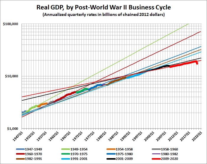
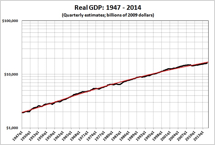
Real GDP (in year 2005 dollars) was $319 billion in 1890; it had risen to $13.3 trillion in 2011 — a compound growth rate of about 3.1 percent. But real GDP in 2011 would have been more than $104 trillion had growth continued at an annual rate of 4.9 percent after 1890 (the rate of growth from 1866 through 1890). What happened? The heavy hand of government (at all levels) — especially after 1929 — made itself felt by discouraging work, discouraging the saving that makes investment possible, discouraging innovation, and (even to the extent that innovation persists) discouraging the investments required to bring innovation on line. How? It begins with the diversion of resources to governmental activities, and is compounded by the cumulative disincentivizing effects of taxes, regulations, administrative procedures, statutes, ordinances, executive orders, and judicial decrees.

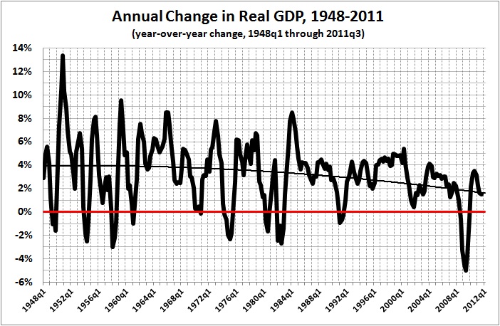
Defenders of big government will say that the rate of growth could not have been sustained at something like 5 percent. But such an assertion, if it is based on anything other than ignorance, is based on a simple, sub-exponential model of growth, where returns on investment are diminishing. This model overlooks the effects of innovation and recombination (the use of previous innovations in new ways). If the model of ever-diminishing growth were correct, the U.S. economy would not have experienced rising growth in the first 20 to 25 years after the end of World War II. No, the defenders of sub-exponential growth must look to the Great Society — and to the continuous expansion of the regulatory-welfare state — if they wish to understand the artificially low rate at which the economy is growing: currently about 2 percent a year.

Despite what I have said here about the deleterious effects of bigger-than-minimal government, there are true believers who maintain that the greater the scope and scale of government, the better and richer America will be. These true believers evidently have not considered the cumulative effect of big government on the incomes and wealth of Americans. As the preceding analysis suggests, those relatively few Americans who would not be better off with minimal government would be the beneficiaries of a pool of charitable giving that is vastly greater than the present pool.

That big government might be harmful, even to the “little people” who are its supposed beneficiaries, is of no account to its worshipers – as long as they run it, advise in the running of it, profit by it, or simply enjoy watching it run roughshod over the lives and fortunes of others. Power and the vicarious enjoyment of power are habit-forming drugs.

The ranks of true believers are peopled such left-wing economists as Brad DeLong, James K. Galbraith, and Paul Krugman. They adhere to and popularize two major rationalizations of big government — the Keynesian fallacy and the myth that government is the same as community.

In “A Keynesian Fantasy Land” I discuss six reasons for the ineffectiveness of Keynesian “stimulus”; in summary:

1. The “leakage” to imports

“Part of the extra spending stimulus fails to stimulate domestic income because as much as 0.3 of the multiplier might leak out through extra imports.” (Anthony de Jasay, “Micro, Macro, and Fantasy Economics,” Library of Economics and Liberty, December 6, 2010)

2. The disincentivizing effects of government borrowing and spending

Even if additional debt does not crowd out private-sector borrowing to finance business expansion, it will nevertheless inhibit investments in business expansion. This inhibiting effect is compounded by the reasonable expectation that many items in a “stimulus” package will become permanent fixtures in the government’s budget

3. The timing-targeting problem

The lag between the initial agitation for “stimulus” and its realization. In the extreme, the lag can be so great as to have no effect other than to divert employed resources from private to government uses. But even where there is a relatively brief lag, “stimulus” spending is essentially wasted if the result is simply to divert already employed resources from private to government uses.

4. Inadequate Aggregate Demand (AD) is a symptom, not a cause

A drop in AD usually is caused by an exogenous event, and that exogenous event usually is a credit crisis. Pumping money into the economy — especially when it results in the bidding up the prices of already employed resources — does not reinflate the punctured credit bubble that caused the slowdown.

5. Inequity, moral hazard, and their consequences

Favorable treatment of defaulters and failing companies generates considerable popular resentment, which — in the present instance — has found a vocal and politically potent outlet in the Tea Party movement. Favorable treatment of defaulters and failing companies also creates moral hazard; that is, it encourage unwise risk-taking that can (and probably will) spark future crises, leading the government to assume more obligations and impose more regulations, in a futile effort to change human nature.

6. The human factor

Those who cling to the Keynesian multiplier would like the world to comply with it. But the world does not because it is filled with people, whose behavior is not determined (or described) by a simplistic model but by their responses to incentives, their political predispositions, their informed and reasonable skepticism about the consequences of government intervention in economic matters, and — above all else — their fallibility.

In truth, the Keynesian multiplier is a mathematical fiction, as explained here, and government spending is in fact destructive of economic growth, as discussed here and in some of the posts listed at the end.

“We owe it to ourselves” is a phrase used by Paul Krugman (among others on the left). It is a variant of the stock rationale for socializing gains and losses: “We’re all in this together.” As if the citizens of the United States were members of an extraordinarily large community, with a perpetual town-hall meeting conducted by the government of the United States.

Consider the intellectual dishonesty of Krugman’s claim that “we” owe the debt of the U.S. government to “ourselves.” Who are “we”? If government borrows money and spends it on goodies for Congressman X, Y, and Z’s districts, how do I get my cut? Or does the happiness generated in Congressman X, Y, and Z’s districts simply radiate in waves across the country, eventually reaching me and making me feel better?

If the borrowed money makes (some) people in Congressman X, Y, and Z’s districts better off, why is it that “we” (i.e. the rest of us and/or our descendants) end up repaying the debt that made those others better off? I do not understand how I “owe it to myself” when (a) I didn’t ask to borrow the money and (b) I gained nothing as a result of the borrowing.

You might claim that my personal wishes are of no account because Congress and the president are duly elected by majorities of voters. But that is tantamount to saying that Congress and the president possess a kind of omniscient super-consciousness that somehow overrides the harm, hate, and discontent that flow from their acts.

The left succeeds, in large part, because apologists for big government — from Krugman to Obama — are skillful practitioners of slippery logic. An assumption here, an assumption there, and government spending is made out to be a source of enrichment. The hard truth is that government spending — and the big government that it supports — is the source of America’s impending impoverishment.

Government in Macroeconomic Perspective

Posted on October 8, 2012 by Loquitur Veritatem

I. INTRODUCTION

A nation’s aggregate economic activity usually is measured by its Gross Domestic Product (GDP). I accept GDP as an aggregate, monetary measure of national output. But it is impossible to sum the true value of the myriad economic transactions that GDP is supposed to represent because each transaction means something different to the participants in the transaction; that is, the true value of economic goods is subjective. (See, for example, Peter Boettke’s “Austrian School of Economics,” at The Concise Encyclopedia of Economics., and my posts, “Subjective Value: A Proof by Example” and “Microeconomics and Macroeconomics.”)

GDP, nevertheless, affords a rough measure of the general level of a nation’s material well-being. All things being the same, a large fraction of a nation’s citizens — but certainly not all of them — will be better off materially if GDP is growing and worse off if it is shrinking. But no one who is paying attention to the state of the nation should mistake material progress for real progress. (See, for example, “I Want My Country Back.”)

The usual way of representing GDP is called the expenditure method. In simple form, it expresses GDP this way:

GDP = private consumption + gross investment + government spending + (exports – imports), or

GDP = C + I + G + (X – M)

Note: “Gross” means that GDP measures production regardless of the various uses to which that production can be put. Production can be used for immediate consumption, for investment in new fixed assets or inventories, or for replacing depreciated fixed assets. “Domestic” means that GDP measures production that takes place within the country’s borders. In the expenditure-method equation given above, the exports-minus-imports term is necessary in order to null out expenditures on things not produced in the country (imports) and add in things produced but not sold in the country (exports). (Taken from “Gross domestic product” at Wikipedia. See also Mack Ott’s “National Income Accounts” at The Concise Encyclopedia of Economics.)

This equation has become so familiar that its correctness is taken for granted. But a bit of reflection reveals it as a model of inconsistency. The dichotomy between consumption and investment is sensible. But the goods acquired and sold in international trade are of the same two types; there is no reason to segregate them from consumption and investment. This is especially true because the sum of consumption and investment is greater than it would be in the absence of international trade. Government, on the other hand, is a net consumer of economic output, not a net producer of it, as the “+ G” term might suggest.

With that background, I will offer an alternative to the standard expenditure method of describing GDP. The journey is step-wise: from a closed economy without international trade or government to an economy with international trade, but without government, to an economy with both international trade and government. Along the way, I fully acknowledge the importance of government as a contributor to GDP, as long as its role is to foster beneficial exchange by maintaining the rule of law and defending Americans from predators, at home and abroad.

That said, government activities (as reflected in total government spending) have led to an economy that produces a small fraction of its potential output. And yet, the true believers in big government seek to make it larger and ever more destructive. I expand on these points at length in Part II, An Alternative Expenditure Model; Part III, The High Cost of Big Government; and Part IV, The Heart of the Problem: Big-Government Worship and Pseudo-Intellectualism. (Continued below the fold.) Continue reading →

The Stock Market as a Leading Indicator of GDP

Posted on September 18, 2012 by Loquitur Veritatem

Stock prices are notoriously volatile, even when measured by a broad index like the S&P Composite. You might think that the S&P Composite is sensitive to broad changes in economic activity, as measured by GDP, for instance. But, as it turns out the S&P Composite, despite its volatility, is a leading indicator of GDP.

I begin with this graph:

Sources: The index of real GDP is derived from estimates of real GDP available at MeasuringWorth.com. The index of the value of the S&P Composite index is derived from Robert Shiller’s data set at http://www.econ.yale.edu/~shiller/data/ie_data.xls.

It is not apparent in the preceding graph, but GDP lags the S&P Composite. The correlation between the percentage change in real GDP and the percentage change in the real S&P composite in the same year is 0.43 (r-squared = .19). The correlation between the change in GDP and the change in the S&P a year earlier is 0.36 (r-squared = 0.13). That correlation is considerably stronger than the correlation between the change in GDP and the change in the S&P a year later (-0.10; r-squared = 0.01), which suggests that the S&P index is a leading indicator of GDP, not the the other way around.

In graphs:

Notes: Both correlations are significant at the 0.1-percent level. The years 1941-1946 are omitted because of the abrupt and largely artificial changes in GDP that arose when the U.S. government commandeered the economy and diverted vast resources to the war effort during World War II.

It seems unnecessary to point out that the correlations are not strong enough to derive precise predictions of GDP from changes in the S&P. However, one could do worse than rely on simple correlations, given the poor track record of complex macroeconomic models (e.g., see this).

It is unsurprising that the stock market has been heading downward since 2000 (despite occasional rallies). Investors know that economic growth is sagging under the pressure of government spending and regulation.

The Burden of Government

Posted on March 20, 2012 by Loquitur Veritatem

When the state is more than a “night watchman,” its cost and intrusiveness diminish liberty and prosperity. (See this and this, for example.) Thus it has come to this: Government takes far more from productive Americans than it returns to them in the form of protection from foreign and domestic predators.

This point is overlooked by the keepers of national-income accounts. To them, government spending (which properly includes so-called transfer payments) adds to GDP. In fact, it detracts from GDP. It is a tax on the output of the private sector. The following graph indicates the size of the tax and its growth with time.

Sources: See footnote.

Some observations:

In 2010, the average output of a private worker was worth $114,000; government confiscated 40 percent of that output, leaving $68,000 in the private sector. (These estimates do not reflect the regulatory burden, which brings the total cost of government to about 50 percent of GDP.)

The direct burden of government spending nearly doubled from 1950 to 2010, rising from 23 percent to 40 percent of the average private employee’s output.

As indicated by the trend lines, real output per worker rose at the rate of $1,125 a year, but only $645 of each year’s increment remained in the private sector. In other words, government spent 43 percent of every additional dollar’s worth of real output per worker.

* * *

Sources:

Estimates of GDP in year 2005 dollars are from the feature “What Was the U.S GDP Then?” at MeasuringWorth.com.

Estimates of government spending (federal, State, and local) are from Statistical Abstracts of the United States, Colonial Times to 1970: Part 2. Series Y 533-566. Federal, State, and Local Government Expenditures, by Function; and the Bureau of Economic Analysis (BEA), Table 3.1. Government Current Receipts and Expenditures (lines 34, 35). The BEA tables are available here.

I estimated private-sector employment by subtracting the number of civilian government employees from the total number of employed persons in the civilian labor force. Government employment figures come from the 2012 Statistical Abstract, Historical Statistics, No. HS–46. Governmental Employment and Payrolls: 1946 to 2001, and the Bureau of Labor Statistics, Series CES9000000001: Employment, Hours, and Earnings from the Current Employment Statistics survey (National), available here. Total civilian employment is from BLS Series LNS12000000, available here.

The Commandeered Economy

Posted on December 24, 2011 by Loquitur Veritatem

Government spending — federal, State, and local — represents the confiscation of resources from the private sector. Any reasonable measure of government spending includes transfer payments (mainly Social Security, Medicare, and Medicaid), which represent income that is taken from persons who earn it and given to persons who do not earn it.

Here is an overview of the patterns of government spending from 1929 through the third quarter of 2011:

Derived from Bureau of Economic Analysis, National Income and Product Accounts, Tables 1.1.5 (lines 1, 21-25), 3.1 (line 17), and 3.2 (line 22).

Total captures all outlays by the federal government and State and local governments for all purposes, including transfer payments. Total non-defense is simply total spending less defense spending. Federal covers all outlays by the federal government, including transfer payments. State & local represents just that. Transfer payments by all governments are driven mainly by outlays for Social Security, Medicare, and Medicaid, which in 2010 accounted for 71 percent of all government spending on “social benefits.” Next is defense, which has been driven mainly by war and the prospect of war. Finally, there is federal non-defense, which is exclusive of transfer payments. This spending enables the federal bureaucracy to perform its non-defense, micromanagement functions: from controlling interest rates and the money supply to regulating the processes and products of America’s businesses to enforcing various forms of discrimination to rewarding well-connected interest groups, and so on into the dark night of fascism.

The rise of government spending began with the onset of the Depression, which saw the federal government supplant State and local governments as the main source of outlays. World War II interrupted but did not break the rising trend in non-defense spending, which has been driven by increases in transfer payments — especially since the inception of Medicare and Medicaid in 1965.

In 1929, on the eve of the Great Depression, government spending of all kinds amounted to 10 percent of GDP, and less than 1 percent of GDP was absorbed by transfer payments. In 1947, following demobilization from World War II, government spending of all kinds was 20 percent of GDP, including 5 percent for transfer payments. Now, total spending consumes about 36 percent of GDP, and transfer payments about 16 percent. All in all, post-World War II spending reflects the dominance of government in the everyday lives of Americans. About 31 percent of GDP goes to non-defense spending by the federal government and State and local governments.

Defense spending — a favored target of “liberals” and pseudo-libertarians — is not where the money is. The stability of total government spending as a percentage of GDP from the end of the Vietnam War until 9/11 was bought by short-changing defense, except during the 1980s. Despite 9/11 and the shallow display of unity that followed it, too many Americans have forgotten the main lessons of World War II and the Cold War: Victory and deterrence do not come cheaply. And yet, since 1950, when defense spending reached its post-war nadir, it has lagged far behind the growth of government spending and transfer payments (which, illogically, have soared despite significant real growth in GDP):

Derived from sources cited above, by applying the implicit GDP deflator used to compute GDP in chained 2005 dollars (here).

In addition to the burden of non-defense spending,* there is the large and growing burden of regulatory compliance: about $1.1 trillion in 2004, or 10 percent of GDP. In other words, government now absorbs or controls almost one-half of the nation’s economic output.

Additionally, however, there is the hidden cost of output forgone because taxes and regulations have discouraged those behaviors that cause economic growth (e.g., hard work, capital formation, innovation, and entrepreneurship). I have estimated that were it not for those disincentives GDP would have grown to more than three times its present level.

The iceberg, once again, proves to be vastly larger than its visible tip. In Bastiat‘s words,

a law produces not only one effect, but a series of effects. Of these effects, the first alone is immediate; it appears simultaneously with its cause; it is seen. The other effects emerge only subsequently; they are not seen; we are fortunate if we foresee them.

The unseen effects — the theft of Americans’ liberty and prosperity — had been foreseen by some (e.g., Tocqueville and Hayek), but ignorance and power-lust prevailed over their prescience.

America’s economy has not been commandeered by the military-industrial complex; it has been commandeered by a far more insidious complex of economically illiterate voters, interest groups, social-engineering “intellectuals,” and power-lusting politicians.

__________

* Defense is a valuable and legitimate “social service,” as I discuss in this post and the posts listed at the end of it. Justice also is a valuable and legitimate “social service,” but spending on police, courts, etc., accounts for only a small fraction of non-defense spending in the U.S.

* * *

On other subjects, see the list at the bottom of “Economic Growth Since World War II.”

Does the CPI Understate Inflation?

Posted on May 28, 2010 by Loquitur Veritatem

REVISED AND RE-DATED

A website called Shadow Government Statistics offers an alternative estimate of inflation. According to SGS, “methodological shifts in government reporting have depressed reported inflation, moving the concept of the CPI away from being a measure of the cost of living needed to maintain a constant standard of living.” (Related post, here.) According to a chart at the linked page, year-over-year inflation is now about 9 percent, as opposed to the official government figure of about 2 percent.

The claim by SGS has merit, and not only because the definition of inflation has shifted. Specifically:

Government spending (at all levels) rose by 6 percentage points between 1980 and 2009. (See the graph at this post.)

Most government spending is inherently inflationary.

The inherently inflationary nature of government spending can be grasped by considering the case where government spending is financed by taxes:

Suppose that in the absence of government the GDP of the United States would be, as it is today, about $15 trillion. (Actually, as I show here, GDP would be a lot more than today’s $15 trillion were government to do nothing more than provide defense and justice.)

Suppose, further, that a bunch of governors arrives on the scene one fine day to announce: “You Americans need our services, so we’re going to tax you $5 trillion in order to provide things that we want you to have.” About 20 percent of the $5 trillion — the money spent on defense and justice — will be of value to almost everyone because (among other things) it protects economic activity. But most of the things our governors wants us to have — a hodge-podge of programs and regulations — will be valued mainly by those governors (i.e., politicians and bureaucrats) and narrow constituencies. The hodge-podge of programs and regulations, along with our governors’ habit of taxing success, raises the real price of government to far more than the $5 trillion shown in our national income accounts.

Our governors’ “generous” confiscation of $5 trillion has the same effect as if the producers of $5 trillion worth of real (non-government) goods and services walk off the job. More accurately, it’s as if they walk off the job and begin to vandalize their capital (homes, commercial buildings, computer networks, etc.). Specifically, according to the chairwoman of Obama’s Council of Economic Advisers, tax increases have a multiplier effect of about 3 (i.e., every dollar of a tax increase yields a 3-fold decrease in GDP). Another economist estimates that the supply of labor declines by 1.9 percent in response to a 1 percent cut in wages (a tax is equivalent to a cut in wages). Even transfer-payment schemes (e.g., Social Security) have a negative economic effect because they penalize producers for the benefit of non-producers.

Despite the reduction in real output that accompanies government,our governors pretend that they are producing $5 trillion worth of services, so (1) they levy taxes for those services, most of which taxes fall on the productive sector, and (2) they pay the producers of government services (government employees and contractors) with those taxes.

In sum, government pays the producers of government services in “empty dollars,” which those producers then try to spend on real output. And so we have $15 trillion chasing $10 trillion worth of real goods and services.

That’s real inflation. No deficit spending necessary. And it happens every time our governors commandeer additional resources, thus widening the gap between what the productive sector could produce and what it actually produces.

What if government were to borrow the $5 trillion instead of imposing $5 trillion in taxes? Borrowing doesn’t change the outcome, just the way we get there. There is still $15 trillion chasing real output of $10 trillion.

Now, not all of that government spending is inherently inflationary. The protection of citizens and their property from foreign and domestic predators (defense and justice) is essential to economic growth and the orderly functioning of free markets. Government spending on defense and justice currently accounts for 8 percent of GDP, whereas government spending (at all levels) currently accounts for 36 percent of GDP. Let’s say, for the sake of argument, (1) that the “right” level of government spending is 10 percent of GDP (the level that obtained in the early 1900s), (2) that the 10 percent is funded by a system of taxes which isn’t punitive toward investors and entrepreneurs (e.g., a single, flat, tax rate), and (3) that the 10 percent is not accompanied by burdensome regulations. Even in the absence of punitive taxes and burdensome regulations, the increase in government spending from 10 to 36 percent of GDP caused prices to rise by 25 percent. Inflation of 25 percent, when spread over 80 years and more, may seem inconsequential. But it is real — real theft, that is.

Moreover, the growth of government spending has been accompanied by punitive taxes and burdensome regulations. As a result, real GDP is 68 percent below its potential. In other words, in the absence of the regulatory-welfare state, real GDP would be more than 3 times its present level.

Visible inflation is bad enough; invisible inflation is a real killer.

Politics and Prosperity

“Government is a disease masquerading as its own cure.”

Tag Archives: GDP

GDP Update

The Economic Damage of COVID-19: A Preliminary Assessment

GDP Trivia

The Real Burden of Government (II)

Let’s Not Get Too Excited about Recent GDP Growth

Vulgar Keynesianism and Capitalism

Why Are Interest Rates So Low?

Keynesianism: Upside-Down Economics in the Collectivist Cause

Government in Macroeconomic Perspective

The Stock Market as a Leading Indicator of GDP

The Burden of Government

The Commandeered Economy

Does the CPI Understate Inflation?

Share this:

Like this:

Share this:

Like this:

Share this:

Like this:

Share this:

Like this:

Share this:

Like this:

Share this:

Like this:

Share this:

Like this:

Share this:

Like this:

Share this:

Like this:

Share this:

Like this:

Share this:

Like this:

Share this:

Like this:

Share this:

Like this:

Share this:

Like this:

Share this:

Like this: