COVID-19 and Probability

This was posted by a Facebook “friend” (who is among many on FB who seem to believe that figuratively hectoring like-minded friends on FB will instill caution among the incautious):

The point I want to make here isn’t about COVID-19, but about probability. It’s a point that I’ve made many times, but the image captures it perfectly. Here’s the point:

When an event has more than one possible outcome, a single trial cannot replicate the average outcome of a large number of trials (replications of the event).

It follows that the average outcome of a large number of trials — the probability of each possible outcome — cannot occur in a single trial.

It is therefore meaningless to ascribe a probability to any possible outcome of a single trial.

Suppose you’re offered a jelly bean from a bag of 100 jelly bean, and are told that two of the jelly beans contain a potentially fatal poison. Do you believe that you have only a 2-percent chance of being poisoned, and would you bet accordingly? Or do you believe, correctly, that you might choose a poisoned jelly bean, and that the “probability” of choosing a poisoned one is meaningless and irrelevant if you want to be certain of surviving the trial at hand (choosing a jelly bean or declining the offer). That is, would you bet (your life) against choosing a poisoned jelly bean?

I have argued (futilely) with several otherwise smart persons who would insist on the 2-percent interpretation. But I doubt (and hope) that any of them would bet accordingly and then choose a jelly bean from a bag of 100 that contains even a single poisoned one, let alone two. Talk is cheap; actions speak louder than words.

Expressing Certainty (or Uncertainty)

I have waged war on the misuse of probability for a long time. As I say in the post at the link:

A probability is a statement about a very large number of like events, each of which has an unpredictable (random) outcome. Probability, properly understood, says nothing about the outcome of an individual event. It certainly says nothing about what will happen next.

From a later post:

It is a logical fallacy to ascribe a probability to a single event. A probability represents the observed or computed average value of a very large number of like events. A single event cannot possess that average value. A single event has a finite number of discrete and mutually exclusive outcomes. Those outcomes will not “average out” — only one of them will obtain, like Schrödinger’s cat.

To say that the outcomes will average out — which is what a probability implies — is tantamount to saying that Jack Sprat and his wife were neither skinny nor fat because their body-mass indices averaged to a normal value. It is tantamount to saying that one can’t drown by walking across a pond with an average depth of 1 foot, when that average conceals the existence of a 100-foot-deep hole.

But what about hedge words that imply “probability” without saying it: certain, uncertain, likely, unlikely, confident, not confident, sure, unsure, and the like? I admit to using such words, which are common in discussions about possible future events and the causes of past events. But what do I, and presumably others, mean by them?

Hedge words are statements about the validity of hypotheses about phenomena or causal relationships. There are two ways of looking at such hypotheses, frequentist and Bayesian:

While for the frequentist, a hypothesis is a proposition (which must be either true or false) so that the frequentist probability of a hypothesis is either 0 or 1, in Bayesian statistics, the probability that can be assigned to a hypothesis can also be in a range from 0 to 1 if the truth value is uncertain.

Further, as discussed above, there is no such thing as the probability of a single event. For example, the Mafia either did or didn’t have JFK killed, and that’s all there is to say about that. One might claim to be “certain” that the Mafia had JFK killed, but one can be certain only if one is in possession of incontrovertible evidence to that effect. But that certainty isn’t a probability, which can refer only to the frequency with which many events of the same kind have occurred and can be expected to occur.

A Bayesian view about the “probability” of the Mafia having JFK killed is nonsensical. Even If a Bayesian is certain, based on incontrovertible evidence, that the Mafia had JFK killed, there is no probability attached to the occurrence. It simply happened, and that’s that.

Lacking such evidence, a Bayesian (or an unwitting “man on the street”) might say “I believe there’s a 50-50 chance that the Mafia had JFK killed”. Does that mean (1) there’s some evidence to support the hypothesis, but it isn’t conclusive, or (2) that the speaker would bet X amount of money, at even odds, that incontrovertible evidence (if any) surfaces it will prove that the Mafia had JFK killed? In the first case, attaching a 50-percent probability to the hypothesis is nonsensical; how does the existence of some evidence translate into a statement about the probability of a one-off event that either occurred or didn’t occur? In the second case, the speaker’s willingness to bet on the occurrence of an event at certain odds tells us something about the speaker’s preference for risk-taking but nothing at all about whether or not the event occurred.

What about the familiar use of “probability” (a.k.a., “chance”) in weather forecasts? Here’s my take:

[W]hen you read or hear a statement like “the probability of rain tomorrow is 80 percent”, you should mentally translate it into language like this:

X guesses that Y will (or will not) happen at time Z, and the “probability” that he attaches to his guess indicates his degree of confidence in it.

The guess may be well-informed by systematic observation of relevant events, but it remains a guess. As most Americans have learned and relearned over the years, when rain has failed to materialize or has spoiled an outdoor event that was supposed to be rain-free.

Further, it is true that some things happen more often than other things but

only one thing will happen at a given time and place.

[A] clever analyst could concoct a probability of a person’s being shot by writing an equation that includes such variables as his size, the speed with which he walks, the number of shooters, their rate of fire, and the distance across the shooting range.

What would the probability estimate mean? It would mean that if a very large number of persons walked across the shooting range under identical conditions, approximately S percent of them would be shot. But the clever analyst cannot specify which of the walkers would be among the S percent.

Here’s another way to look at it. One person wearing head-to-toe bullet-proof armor could walk across the range a large number of times and expect to be hit by a bullet on S percent of his crossings. But the hardy soul wouldn’t know on which of the crossings he would be hit.

Suppose the hardy soul became a foolhardy one and made a bet that he could cross the range without being hit. Further, suppose that S is estimated to be 0.75; that is, 75 percent of a string of walkers would be hit, or a single (bullet-proof) walker would be hit on 75 percent of his crossings. Knowing the value of S, the foolhardy fellow offers to pay out $1 million dollars if he crosses the range unscathed — one time — and claim $4 million (for himself or his estate) if he is shot. That’s an even-money bet, isn’t it?

No it isn’t….

The bet should be understood for what it is, an either-or-proposition. The foolhardy walker will either lose $1 million or win $4 million. The bettor (or bettors) who take the other side of the bet will either win $1 million or lose $4 million.

As anyone with elementary reading and reasoning skills should be able to tell, those possible outcomes are not the same as the outcome that would obtain (approximately) if the foolhardy fellow could walk across the shooting range 1,000 times. If he could, he would come very close to breaking even, as would those who bet against him.

I omitted from the preceding quotation a sentence in which I used “more likely”:

If a person walks across a shooting range where live ammunition is being used, he is more likely to be killed than if he walks across the same patch of ground when no one is shooting.

Inasmuch as “more likely” is a hedge word, I seem to have contradicted my own position about the probability of a single event, such as being shot while walking across a shooting range. In that context, however, “more likely” means that something could happen (getting shot) that wouldn’t happen in a different situation. That’s not really a probabilistic statement. It’s a statement about opportunity; thus:

  • Crossing a firing range generates many opportunities to be shot.
  • Going into a crime-ridden neighborhood certainly generates some opportunities to be shot, but their number and frequency depends on many variables: which neighborhood, where in the neighborhood, the time of day, who else is present, etc.
  • Sitting by oneself, unarmed, in a heavy-gauge steel enclosure generates no opportunities to be shot.

The “chance” of being shot is, in turn, “more likely”, “likely”, and “unlikely” — or a similar ordinal pattern that uses “certain”, “confident”, “sure”, etc. But the ordinal pattern, in any case, can never (logically) include statements like “completely certain”, “completely confident”, etc.

An ordinal pattern is logically valid only if it conveys the relative number of opportunities to attain a given kind of outcome — being shot, in the example under discussion.

Ordinal statements about different types of outcome are meaningless. Consider, for example, the claim that the probability that the Mafia had JFK killed is higher than (or lower than or the same as) the probability that the moon is made of green cheese. First, and to repeat myself for the nth time, the phenomena in question are one-of-a-kind and do not lend themselves to statements about their probability, nor even about the frequency of opportunities for the occurrence of the phenomena. Second, the use of “probability” is just a hifalutin way of saying that the Mafia could have had a hand in the killing of JFK, whereas it is known (based on ample scientific evidence, including eye-witness accounts) that the Moon isn’t made of green cheese. So the ordinal statement is just a cheap rhetorical trick that is meant to (somehow) support the subjective belief that the Mafia “must” have had a hand in the killing of JFK.

Similarly, it is meaningless to say that the “average person” is “more certain” of being killed in an auto accident than in a plane crash, even though one may have many opportunities to die in an auto accident or a plane crash. There is no “average person”; the incidence of auto travel and plane travel varies enormously from person to person; and the conditions that conduce to fatalities in auto travel and plane travel vary just as enormously.

Other examples abound. Be on the lookout for them, and avoid emulating them.

Ford, Kavanaugh, and Probability

I must begin by quoting the ever-quotable Theodore Dalrymple. In closing a post in which he addresses (inter alia) the high-tech low-life lynching of Brett Kavanaugh, he writes:

The most significant effect of the whole sorry episode is the advance of the cause of what can be called Femaoism, an amalgam of feminism and Maoism. For some people, there is a lot of pleasure to be had in hatred, especially when it is made the meaning of life.

Kavanaugh’s most “credible” accuser — Christine Blasey Ford (CBF) — was incredible (in the literal meaning of the word) for many reasons, some of which are given in the items listed at the end of “Where I Stand on Kavanaugh“.

Arnold Kling gives what is perhaps the best reason for believing Kavanaugh’s denial of CBF’s accusation, a reason that occurred to me at the time:

[Kavanaugh] came out early and emphatically with his denial. This risked having someone corroborate the accusation, which would have irreparably ruined his career. If he did it, it was much safer to own it than to attempt to get away with lying about it. If he lied, chances are he would be caught–at some point, someone would corroborate her story. The fact that he took that risk, along with the fact that there was no corroboration, even from her friend, suggests to me that he is innocent.

What does any of this have to do with probability? Kling’s post is about the results of a survey conducted by Scott Alexander, the proprietor of Slate Star Codex. Kling opens with this:

Scott Alexander writes,

I asked readers to estimate their probability that Judge Kavanaugh was guilty of sexually assaulting Dr. Ford. I got 2,350 responses (thank you, you are great). Here was the overall distribution of probabilities.

… A classical statistician would have refused to answer this question. In classical statistics, he is either guilty or he is not. A probability statement is nonsense. For a Bayesian, it represents a “degree of belief” or something like that. Everyone who answered the poll … either is a Bayesian or consented to act like one.

As a staunch adherent of the classical position (though I am not a statistician), I agree with Kling.

But the real issue in the recent imbroglio surrounding Kavanaugh wasn’t the “probability” that he had committed or attempted some kind of assault on CBF. The real issue was the ideological direction of the Supreme Court:

  1. With the departure of Anthony Kennedy from the Court, there arose an opportunity to secure a reliably conservative (constitutionalist) majority. (Assuming that Chief Justice Roberts remains in the fold.)
  2. Kavanaugh is seen to be a reliable constitutionalist.
  3. With Kavanaugh in the conservative majority, the average age of that majority would be (and now is) 63; whereas, the average age of the “liberal” minority is 72, and the two oldest justices (at 85 and 80) are “liberals”.
  4. Though the health and fitness of individual justices isn’t well known, there are more opportunities in the coming years for the enlargement of the Court’s conservative wing than for the enlargement of its “liberal” wing.
  5. This is bad news for the left because it dims the prospects for social and economic revolution via judicial decree — a long-favored leftist strategy. In fact, it brightens the prospects for the rollback of some of the left’s legislative and judicial “accomplishments”.

Thus the transparently fraudulent attacks on Brett Kavanaugh by desperate leftists and “tools” like CBF. That is to say, except for those who hold a reasoned position (e.g., Arnold Kling and me), one’s stance on Kavanaugh is driven by one’s politics.

Scott Alexander’s post supports my view:

Here are the results broken down by party (blue is Democrats, red is Republicans):

And here are the results broken down by gender (blue is men, pink is women):

Given that women are disproportionately Democrat, relative to men, the second graph simply tells us the same thing as the first graph: The “probability” of Kavanaugh’s “guilt” is strongly linked to political persuasion. (I am heartened to see that a large chunk of the female population hasn’t succumbed to Femaoism.)

Probability, in the proper meaning of the word, has nothing to do with question of Kavanaugh’s “guilt”. A feeling or inclination isn’t a probability, it’s just a feeling or inclination. Putting a number on it is false quantification. Scott Alexander should know better.

The Probability That Something Will Happen

A SINGLE EVENT DOESN’T HAVE A PROBABILITY

A believer in single-event probabilities takes the view that a single flip of a coin or roll of a dice has a probability. I do not. A probability represents the frequency with which an outcome occurs over the very long run, and it is only an average that conceals random variations.

The outcome of a single coin flip can’t be reduced to a percentage or probability. It can only be described in terms of its discrete, mutually exclusive possibilities: heads (H) or tails (T). The outcome of a single roll of a die or pair of dice can only be described in terms of the number of points that may come up, 1 through 6 or 2 through 12.

Yes, the expected frequencies of H, T, and and various point totals can be computed by simple mathematical operations. But those are only expected frequencies. They say nothing about the next coin flip or dice roll, nor do they more than approximate the actual frequencies that will occur over the next 100, 1,000, or 10,000 such events.

Of what value is it to know that the probability of H is 0.5 when H fails to occur in 11 consecutive flips of a fair coin? Of what value is it to know that the probability of rolling a  7 is 0.167 — meaning that 7 comes up every 6 rolls, on average — when 7 may not appear for 56 consecutive rolls? These examples are drawn from simulations of 10,000 coin flips and 1,000 dice rolls. They are simulations that I ran once, not simulations that I cherry-picked from many runs. (The Excel file is at https://drive.google.com/open?id=1FABVTiB_qOe-WqMQkiGFj2f70gSu6a82. Coin flips are at the first tab, dice rolls are at the second tab.)

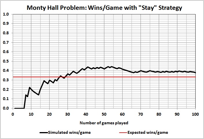
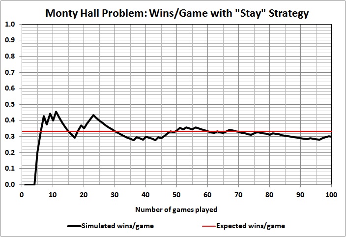
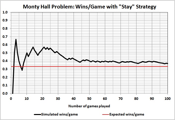
Let’s take another example, one that is more interesting and has generated much controversy of the years. It’s the Monty Hall problem,

a brain teaser, in the form of a probability puzzle, loosely based on the American television game show Let’s Make a Deal and named after its original host, Monty Hall. The problem was originally posed (and solved) in a letter by Steve Selvin to the American Statistician in 1975…. It became famous as a question from a reader’s letter quoted in Marilyn vos Savant’s “Ask Marilyn” column in Parade magazine in 1990 … :

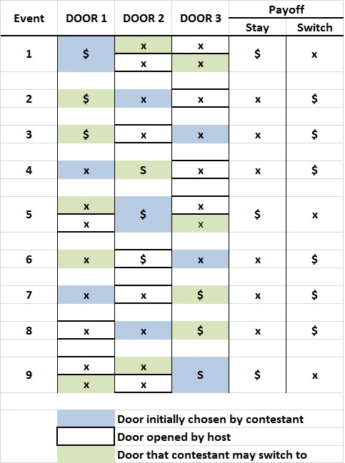
Suppose you’re on a game show, and you’re given the choice of three doors: Behind one door is a car; behind the others, goats. You pick a door, say No. 1, and the host, who knows what’s behind the doors, opens another door, say No. 3, which has a goat. He then says to you, “Do you want to pick door No. 2?” Is it to your advantage to switch your choice

Vos Savant’s response was that the contestant should switch to the other door…. Under the standard assumptions, contestants who switch have a 2/3 chance of winning the car, while contestants who stick to their initial choice have only a 1/3 chance.

Vos Savant’s answer is correct, but only if the contestant is allowed to play an unlimited number of games. A player who adopts a strategy of “switch” in every game will, in the long run, win about 2/3 of the time (explanation here). That is, the player has a better chance of winning if he chooses “switch” rather than “stay”.

Read the preceding paragraph carefully and you will spot the logical defect that underlies the belief in single-event probabilities: The long-run winning strategy (“switch”) is transformed into a “better chance” to win a particular game. What does that mean? How does an average frequency of 2/3 improve one’s chances of winning a particular game? It doesn’t. Game results are utterly random; that is, the average frequency of 2/3 has no bearing on the outcome of a single game.

I’ll try to drive the point home by returning to the coin-flip game, with money thrown into the mix. A $1 bet on H means a gain of $1 if H turns up, and a loss of $1 if T turns up. The expected value of the bet — if repeated over a very large number of trials — is zero. The bettor expects to win and lose the same number of times, and to walk away no richer or poorer than when he started. And for a very large number of games, the better will walk away approximately (but not necessarily exactly) neither richer nor poorer than when he started. How many games? In the simulation of 10,000 games mentioned earlier, H occurred 50.6 percent of the time. A very large number of games is probably at least 100,000.

Let us say, for the sake of argument, that a bettor has played 100,00 coin-flip games at $1 a game and come out exactly even. What does that mean for the play of the next game? Does it have an expected value of zero?

To see why the answer is “no”, let’s make it interesting and say that the bet on the next game — the next coin flip — is $10,000. The size of the bet should wonderfully concentrate the bettor’s mind. He should now see the situation for what it really is: There are two possible outcomes, and only one of them will be realized. An average of the two outcomes is meaningless. The single coin flip doesn’t have a “probability” of 0.5 H and 0.5 T and an “expected payoff” of zero. The coin will come up either H or T, and the bettor will either lose $10,000 or win $10,000.

To repeat: The outcome of a single coin flip doesn’t have an expected value for the bettor. It has two possible values, and the bettor must decide whether he is willing to lose $10,000 on the single flip of a coin.

By the same token (or coin), the outcome of a single roll of a pair of dice doesn’t have a 1-in-6 probability of coming up 7. It has 36 possible outcomes and 11 possible point totals, and the bettor must decide how much he is willing to lose if he puts his money on the wrong combination or outcome.

In summary, it is a logical fallacy to ascribe a probability to a single event. A probability represents the observed or computed average value of a very large number of like events. A single event cannot possess that average value. A single event has a finite number of discrete and mutually exclusive possible outcomes. Those outcomes will not “average out” in that single event. Only one of them will obtain, like Schrödinger’s cat.

To say or suggest that the outcomes will average out — which is what a probability implies — is tantamount to saying that Jack Sprat and his wife were neither skinny nor fat because their body-mass indices averaged to a normal value. It is tantamount to saying that one can’t drown by walking across a pond with an average depth of 1 foot, when that average conceals the existence of a 100-foot-deep hole.

It should go without saying that a specific event that might occur — rain tomorrow, for example — doesn’t have a probability.

WHAT ABOUT THE PROBABILITY OF PRECIPITATION?

Weather forecasters (meteorologists) are constantly saying things like “there’s an 80-percent probability of precipitation (PoP) in __________ tomorrow”. What do such statements mean? Not much:

It is not surprising that this issue is difficult for the general public, given that it is debated even within the scientific community. Some propose a “frequentist” interpretation: there will be at least a minimum amount of rain on 80% of days with weather conditions like they are today. Although preferred by many scientists, this explanation may be particularly difficult for the general public to grasp because it requires regarding tomorrow as a class of events, a group of potential tomorrows. From the perspective of the forecast user, however, tomorrow will happen only once. A perhaps less abstract interpretation is that PoP reflects the degree of confidence that the forecaster has that it will rain. In other words, an 80% chance of rain means that the forecaster strongly believes that there will be at least a minimum amount of rain tomorrow. The problem, from the perspective of the general public, is that when PoP is forecasted, none of these interpretations is specified.

There are clearly some interpretations that are not correct. The percentage expressed in PoP neither refers directly to the percent of area over which precipitation will fall nor does it refer directly to the percent of time precipitation will be observed on the forecast day Although both interpretations are clearly wrong, there is evidence that the general public holds them to varying degrees. Such misunderstandings are critical because they may affect the decisions that people make. If people misinterpret the forecast as percent time or percent area, they maybe more inclined to take precautionary action than are those who have the correct probabilistic interpretation, because they think that it will rain somewhere or some time tomorrow. The negative impact of such misunderstandings on decision making, both in terms of unnecessary precautions as well as erosion in user trust, could well eliminate any potential benefit of adding uncertainty information to the forecast. [Susan Joslyn, Nimor Nadav-Greenberg, and Rebecca M. Nichols, “Probability of Precipitations: Assessment and Enhancement of End-User Understanding“, Journal of the American Meteorological Society, February 2009, citations omitted]

The frequentist interpretation is close to be correct, but it still involves a great deal of guesswork. Rainfall in a particular location is influenced by many variables (e.g., atmospheric pressure, direction and rate of change of atmospheric pressure, ambient temperature, local terrain, presence or absence of bodies of water, vegetation, moisture content of the atmosphere, height of clouds above the terrain, depth of cloud cover). It is nigh unto impossible to say that today’s (or tomorrow’s or next week’s) weather conditions are like (or will be like) those that in the past resulted in rainfall in a particular location 80 percent of the time.

That leaves the Bayesian interpretation, in which the forecaster combines some facts (e.g., the presence or absence of a low-pressure system in or toward the area, the presence or absence of a flow of water vapor in or toward the area) with what he has observed in the past to arrive at a guess about future weather. He then attaches a probability to his guess to indicate the strength of his confidence in it.

Thus:

Bayesian probability represents a level of certainty relating to a potential outcome or idea. This is in contrast to a frequentist probability that represents the frequency with which a particular outcome will occur over any number of trials.

An event with Bayesian probability of .6 (or 60%) should be interpreted as stating “With confidence 60%, this event contains the true outcome”, whereas a frequentist interpretation would view it as stating “Over 100 trials, we should observe event X approximately 60 times.”

And thus:

The Bayesian approach to learning is based on the subjective interpretation of probability. The value of the proportion p is unknown, and a person expresses his or her opinion about the uncertainty in the proportion by means of a probability distribution placed on a set of possible values of p.

It is impossible to attach a probability — as properly defined in the first part of this article — to something that hasn’t happened, and may not happen. So when you read or hear a statement like “the probability of rain tomorrow is 80 percent”, you should mentally translate it into language like this:

X guesses that Y will (or will not) happen at time Z, and the “probability” that he attaches to his guess  indicates his degree of confidence in it.

The guess may be well-informed by systematic observation of relevant events, but it remains a guess. As most Americans have learned and relearned over the years, when rain has failed to materialize or has spoiled an outdoor event that was supposed to be rain-free.

BUT AREN’T SOME THINGS MORE LIKELY TO HAPPEN THAN OTHERS?

Of course. But only one thing will happen at a given time and place.

If a person walks across a shooting range where live ammunition is being used, his is more likely to be killed than if he walks across the same patch of ground when no one is shooting. And a clever analyst could concoct a probability of a person’s being shot by writing an equation that includes such variables as his size, the speed with which he walks, the number of shooters, their rate of fire, and the distance across the shooting range.

What would the probability estimate mean? It would mean that if a very large number of persons walked across the shooting range under identical conditions, approximately S percent of them would be shot. But the clever analyst cannot specify which of the walkers would be among the S percent.

Here’s another way to look at it. One person wearing head-to-toe bullet-proof armor could walk across the range a large number of times and expect to be hit by a bullet on S percent of his crossings. But the hardy soul wouldn’t know on which of the crossings he would be hit.

Suppose the hardy soul became a foolhardy one and made a bet that he could cross the range without being hit. Further, suppose that S is estimated to be 0.75; that is, 75 percent of a string of walkers would be hit, or a single (bullet-proof) walker would be hit on 75 percent of his crossings. Knowing the value of S, the foolhardy fellow offers to pay out $1 million dollars if he crosses the range unscathed — one time — and claim $4 million (for himself or his estate) if he is shot. That’s an even-money bet, isn’t it?

No it isn’t. This situation is exactly analogous to the $10,000 bet on a single coin flip, discussed above. But I will dissect this one in a different way, to the same end.

The bet should be understood for what it is, an either-or-proposition. The foolhardy walker will either lose $1 million or win $4 million. The bettor (or bettors) who take the other side of the bet will either win $1 million or lose $4 million.

As anyone with elementary reading and reasoning skills should be able to tell, those possible outcomes are not the same as the outcome that would obtain (approximately) if the foolhardy fellow could walk across the shooting range 1,000 times. If he could, he would come very close to breaking even, as would those who bet against him.

To put it as simply as possible:

When an event has more than one possible outcome, a single trial cannot replicate the average outcome of a large number of trials (replications of the event).

It follows that the average outcome of a large number of trials — the probability of each possible outcome — cannot occur in a single trial.

It is therefore meaningless to ascribe a probability to any possible outcome of a single trial.

MODELING AND PROBABILITY

Sometimes, when things interact, the outcome of the interactions will conform to an expected value — if that value is empirically valid. For example, if a pot of pure water is put over a flame at sea level, the temperature of the water will rise to 212 degrees Fahrenheit and water molecules will then begin to escape into the air in a gaseous form (steam).  If the flame is kept hot enough and applied long enough, the water in the pot will continue to vaporize until the pot is empty.

That isn’t a probabilistic description of boiling. It’s just a description of what’s known to happen to water under certain conditions.

But it bears a similarity to a certain kind of probabilistic reasoning. For example, in a paper that I wrote long ago about warfare models, I said this:

Consider a five-parameter model, involving the conditional probabilities of detecting, shooting at, hitting, and killing an opponent — and surviving, in the first place, to do any of these things. Such a model might easily yield a cumulative error of a hemibel [a factor of 3], given a twenty five percent error in each parameter.

Mathematically, 1.255 = 3.05. Which is true enough, but also misleadingly simple.

A mathematical model of that kind rests on the crucial assumption that the component probabilities are based on observations of actual events occurring in similar conditions. It is safe to say that the values assigned to the parameters of warfare models, econometric models, sociological models, and most other models outside the realm of physics, chemistry, and other “hard” sciences fail to satisfy that assumption.

Further, a mathematical model yields only the expected (average) outcome of a large number of events occurring under conditions similar to those from which the component probabilities were derived. (A Monte Carlo model merely yields a quantitative estimate of the spread around the average outcome.) Again, this precludes most models outside the “hard” sciences, and even some within that domain.

The moral of the story: Don’t be gulled by a statement about the expected outcome of an event, even when the statement seems to be based on a rigorous mathematical formula. Look behind the formula for an empirical foundation. And not just any empirical foundation, but one that is consistent with the situation to which the formula is being applied.

And when you’ve done that, remember that the formula expresses a point estimate around which there’s a wide — very wide — range of uncertainty. Which was the real point of the passage quoted above. The only sure things in life are death, taxes, and regulation.

PROBABILITY VS. OPPORTUNITY

Warfare models, as noted, deal with interactions among large numbers of things. If a large unit of infantry encounters another large unit of enemy infantry, and the units exchange gunfire, it is reasonable to expect the following consequences:

  • As the numbers of infantrymen increase, more of them will be shot, for a given rate of gunfire.
  • As the rate of gunfire increases, more of the infantrymen will be shot, for a given number of infantrymen.

These consequences don’t represent probabilities, though an inveterate modeler will try to represent them with a probabilistic model. They represent opportunities — opportunities for bullets to hit bodies. It is entirely possible that some bullets won’t hit bodies and some bodies won’t be hit by bullets. But more bullets will hit bodies if there are more bodies in a given space. And a higher proportion of a given number of bodies will be hit as more bullets enter a given space.

That’s all there is to it.

It has nothing to do with probability. The actual outcome of a past encounter is the actual outcome of that encounter, and the number of casualties has everything to do with the minutiae of the encounter and nothing to do with probability. A fortiori, the number of casualties resulting from a possible future encounter would have everything to do with the minutiae of that encounter and nothing to do with probability. Given the uniqueness of any given encounter, it would be wrong to characterize its outcome (e.g., number of casualties per infantryman) as a probability.


Related posts:
Understanding the Monty Hall Problem
The Compleat Monty Hall Problem
Some Thoughts about Probability
My War on the Misuse of Probability
Scott Adams Understands Probability
Further Thoughts about Probability

Further Thoughts about Probability

BACKGROUND

A few weeks ago I posted “A Bayesian Puzzle”. I took it down because Bayesianism warranted more careful treatment than I had given it. But while the post was live at Ricochet (where I cross-posted in September-November), I had an exchange with a reader who is an obdurate believer in single-event probabilities, such as “the probability of heads on the next coin flip is 50 percent” and “the probability of 12 on the next roll of a pair of dice is 1/18”. That wasn’t the first such exchange of its kind that I’ve had; “Some Thoughts about Probability” reports an earlier and more thoughtful exchange with a believer in single-event probabilities.

DISCUSSION

A believer in single-event probabilities takes the view that a single flip of a coin or roll of dice has a probability. I do not. A probability represents the frequency with which an outcome occurs over the very long run, and it is only an average that conceals random variations.

The outcome of a single coin flip can’t be reduced to a percentage or probability. It can only be described in terms of its discrete, mutually exclusive possibilities: heads (H) or tails (T). The outcome of a single roll of a die or pair of dice can only be described in terms of the number of points that may come up, 1 through 6 or 2 through 12.

Yes, the expected frequencies of H, T, and and various point totals can be computed by simple mathematical operations. But those are only expected frequencies. They say nothing about the next coin flip or dice roll, nor do they more than approximate the actual frequencies that will occur over the next 100, 1,000, or 10,000 such events.

Of what value is it to know that the probability of H is 0.5 when H fails to occur in 11 consecutive flips of a fair coin? Of what value is it to know that the probability of rolling a  7 is 0.167 — meaning that 7 comes up every 6 rolls, on average — when 7 may not appear for 56 consecutive rolls? These examples are drawn from simulations of 10,000 coin flips and 1,000 dice rolls. They are simulations that I ran once — not simulations that I cherry-picked from many runs. (The Excel file is at https://drive.google.com/open?id=1FABVTiB_qOe-WqMQkiGFj2f70gSu6a82 — coin flips are on the first tab, dice rolls are on the second tab.)

Let’s take another example, which is more interesting, and has generated much controversy of the years. It’s the Monty Hall problem,

a brain teaser, in the form of a probability puzzle, loosely based on the American television game show Let’s Make a Deal and named after its original host, Monty Hall. The problem was originally posed (and solved) in a letter by Steve Selvin to the American Statistician in 1975…. It became famous as a question from a reader’s letter quoted in Marilyn vos Savant’s “Ask Marilyn” column in Parade magazine in 1990 … :

Suppose you’re on a game show, and you’re given the choice of three doors: Behind one door is a car; behind the others, goats. You pick a door, say No. 1, and the host, who knows what’s behind the doors, opens another door, say No. 3, which has a goat. He then says to you, “Do you want to pick door No. 2?” Is it to your advantage to switch your choice

Vos Savant’s response was that the contestant should switch to the other door…. Under the standard assumptions, contestants who switch have a 2/3 chance of winning the car, while contestants who stick to their initial choice have only a 1/3 chance.

Vos Savant’s answer is correct, but only if the contestant is allowed to play an unlimited number of games. A player who adopts a strategy of “switch” in every game will, in the long run, win about 2/3 of the time (explanation here). That is, the player has a better chance of winning if he chooses “switch” rather than “stay”.

Read the preceding paragraph carefully and you will spot the logical defect that underlies the belief in single-event probabilities: The long-run winning strategy (“switch”) is transformed into a “better chance” to win a particular game. What does that mean? How does an average frequency of 2/3 improve one’s chances of winning a particular game? It doesn’t. As I show here, game results are utterly random; that is, the average frequency of 2/3 has no bearing on the outcome of a single game.

I’ll try to drive the point home by returning to the coin-flip game, with money thrown into the mix. A $1 bet on H means a gain of $1 if H turns up, and a loss of $1 if T turns up. The expected value of the bet — if repeated over a very large number of trials — is zero. The bettor expects to win and lose the same number of times, and to walk away no richer or poorer than when he started. And for a very large number of games, the better will walk away approximately (but not necessarily exactly) neither richer nor poorer than when he started. How many games? In the simulation of 10,000 games mentioned earlier, H occurred 50.6 percent of the time. A very large number of games is probably at least 100,000.

Let us say, for the sake of argument, that a bettor has played 100,00 coin-flip games at $1 a game and come out exactly even. What does that mean for the play of the next game? Does it have an expected value of zero?

To see why the answer is “no”, let’s make it interesting and say that the bet on the next game — the next coin flip — is $10,000. The size of the bet should wonderfully concentrate the bettor’s mind. He should now see the situation for what it really is: There are two possible outcomes, and only one of them will be realized. An average of the two outcomes is meaningless. The single coin flip doesn’t have a “probability” of 0.5 H and 0.5 T and an “expected payoff” of zero. The coin will come up either H or T, and the bettor will either lose $10,000 or win $10,000.

To repeat: The outcome of a single coin flip doesn’t have an expected value for the bettor. It has two possible values, and the bettor must decide whether he is willing to lose $10,000 on the single flip of a coin.

By the same token (or coin), the outcome of a single roll of a pair of dice doesn’t have a 1-in-6 probability of coming up 7. It has 36 possible outcomes and 11 possible point totals, and the bettor must decide how much he is willing to lose if he puts his money on the wrong combination or outcome.

CONCLUSION

It is a logical fallacy to ascribe a probability to a single event. A probability represents the observed or computed average value of a very large number of like events. A single event cannot possess that average value. A single event has a finite number of discrete and mutually exclusive outcomes. Those outcomes will not “average out” — only one of them will obtain, like Schrödinger’s cat.

To say that the outcomes will average out — which is what a probability implies — is tantamount to saying that Jack Sprat and his wife were neither skinny nor fat because their body-mass indices averaged to a normal value. It is tantamount to saying that one can’t drown by walking across a pond with an average depth of 1 foot, when that average conceals the existence of a 100-foot-deep hole.


Related posts:
Understanding the Monty Hall Problem
The Compleat Monty Hall Problem
Some Thoughts about Probability
My War on the Misuse of Probability
Scott Adams Understands Probability

Babe Ruth and the Hot-Hand Hypothesis

According to Wikipedia, the so-called hot-hand fallacy is that “a person who has experienced success with a seemingly random event has a greater chance of further success in additional attempts.” The article continues:

[R]esearchers for many years did not find evidence for a “hot hand” in practice. However, later research has questioned whether the belief is indeed a fallacy. More recent studies using modern statistical analysis have shown that there is evidence for the “hot hand” in some sporting activities.

I won’t repeat the evidence cited in the Wikipedia article, nor will I link to the many studies about the hot-hand effect. You can follow the link and read it all for yourself.

What I will do here is offer an analysis that supports the hot-hand hypothesis, taking Babe Ruth as a case in point. Ruth was a regular position player (non-pitcher) from 1919 through 1934. In that span of 16 seasons he compiled 688 home runs (HR) in 7,649 at-bats (AB) for an overall record of 0.0900 HR/AB. Here are the HR/AB tallies for each of the 16 seasons:

Year HR/AB
1919 0.067
1920 0.118
1921 0.109
1922 0.086
1923 0.079
1924 0.087
1925 0.070
1926 0.095
1927 0.111
1928 0.101
1929 0.092
1930 0.095
1931 0.086
1932 0.090
1933 0.074
1934 0.060

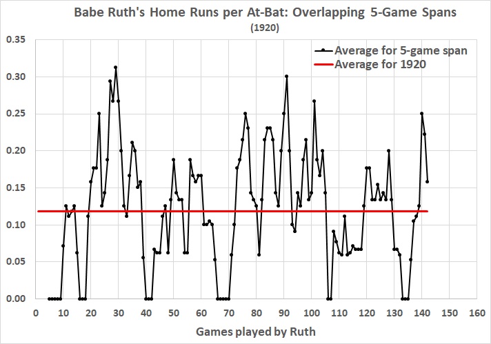
Despite the fame that accrues to Ruth’s 1927 season, when he hit 60 home runs, his best season for HR/AB came in 1920. In 1919, Ruth set a new single-season record with 29 HR. He almost doubled that number in 1920, getting 54 HR in 458 AB for 0.118 HR/AB.

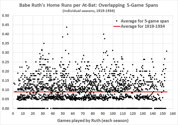
Here’s what that season looks like, in graphical form:

The word for it is “streaky”, which isn’t surprising. That’s the way of most sports. Streaks include not only cold spells but also hot spells. Look at the relatively brief stretches in which Ruth was shut out in the HR department. And look at the relatively long stretches in which he readily exceeded his HR/AB for the season. (For more about the hot and and streakiness, see Brett Green and Jeffrey Zwiebel, “The Hot-Hand Fallacy: Cognitive Mistakes or Equilibrium Adjustments? Evidence from Major League Baseball“, Stanford Graduate School of Business, Working Paper No. 3101, November 2013.)

The same pattern can be inferred from this composite picture of Ruth’s 1919-1934 seasons:

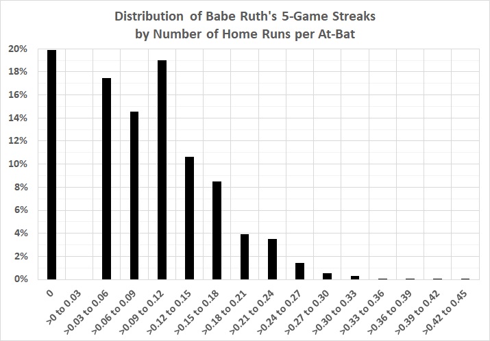
Here’s another way to look at it:

If hitting home runs were a random thing — which they would be if the hot hand were a fallacy — the distribution would be tightly clustered around the mean of 0.0900 HR/AB. Nor would there be a gap between 0 HR/AB and the 0.03 to 0.06 bin. In fact, the gap is wider than that; it goes from 0 to 0.042 HR/AB. When Ruth broke out of a home-run slump, he broke out with a vengeance, because he had the ability to do so.

In other words, Ruth’s hot streaks weren’t luck. They were the sum of his ability and focus (or “flow“); he was “putting it all together”. The flow was broken at times — by a bit of bad luck, a bout of indigestion, a lack of sleep, a hangover, an opponent who “had his number”, etc. But a great athlete like Ruth bounces back and put it all together again and again, until his skills fade to the point that he can’t overcome his infirmities by waiting for his opponents to make mistakes.

The hot hand is the default condition for a great player like a Ruth or a Cobb. The cold hand is the exception until the great player’s skills finally wither. And there’s no sharp dividing line between the likes of Cobb and Ruth and lesser mortals. Anyone who has the ability to play a sport at a professional level (and many an amateur, too) will play with a hot hand from time to time.

The hot hand isn’t a fallacy or a matter of pure luck (or randomness). It’s an artifact of skill.


Related posts:
Flow
Fooled by Non-Randomness
Randomness Is Over-Rated
Luck and Baseball, One More Time
Pseudoscience, “Moneyball,” and Luck
Ty Cobb and the State of Science
The American League’s Greatest Hitters: III

Bayesian Irrationality

I just came across a strange and revealing statement by Tyler Cowen:

I am frustrated by the lack of Bayesianism in most of the religious belief I observe. I’ve never met a believer who asserted: “I’m really not sure here. But I think Lutheranism is true with p = .018, and the next strongest contender comes in only at .014, so call me Lutheran.” The religious people I’ve known rebel against that manner of framing, even though during times of conversion they may act on such a basis.

I don’t expect all or even most religious believers to present their views this way, but hardly any of them do. That in turn inclines me to think they are using belief for psychological, self-support, and social functions.

I wouldn’t expect anyone to say something like “Lutheranism is true with p = .018”. Lutheranism is either true or false. Just as a person on trial is either guilty or innocent. One may have doubts about the truth of Lutheranism or the guilt of a defendant, but those doubts have nothing to do with probability. Neither does Bayesianism.

In defense of probability, I will borrow heavily from myself. According to Wikipedia (as of December 19, 2014):

Bayesian probability represents a level of certainty relating to a potential outcome or idea. This is in contrast to a frequentist probability that represents the frequency with which a particular outcome will occur over any number of trials.

An event with Bayesian probability of .6 (or 60%) should be interpreted as stating “With confidence 60%, this event contains the true outcome”, whereas a frequentist interpretation would view it as stating “Over 100 trials, we should observe event X approximately 60 times.”

Or consider this account:

The Bayesian approach to learning is based on the subjective interpretation of probability.   The value of the proportion p is unknown, and a person expresses his or her opinion about the uncertainty in the proportion by means of a probability distribution placed on a set of possible values of p….

“Level of certainty” and “subjective interpretation” mean “guess.” The guess may be “educated.” It’s well known, for example, that a balanced coin will come up heads about half the time, in the long run. But to say that “I’m 50-percent confident that the coin will come up heads” is to say nothing meaningful about the outcome of a single coin toss. There are as many probable outcomes of a coin toss as there are bystanders who are willing to make a statement like “I’m x-percent confident that the coin will come up heads.” Which means that a single toss doesn’t have a probability, though it can be the subject of many opinions as to the outcome.

Returning to reality, Richard von Mises eloquently explains frequentism in Probability, Statistics and Truth (second revised English edition, 1957). Here are some excerpts:

The rational concept of probability, which is the only basis of probability calculus, applies only to problems in which either the same event repeats itself again and again, or a great number of uniform elements are involved at the same time. Using the language of physics, we may say that in order to apply the theory of probability we must have a practically unlimited sequence of uniform observations. [P. 11]

*     *     *

In games of dice, the individual event is a single throw of the dice from the box and the attribute is the observation of the number of points shown by the dice. In the game of “heads or tails”, each toss of the coin is an individual event, and the side of the coin which is uppermost is the attribute. [P. 11]

*     *     *

We must now introduce a new term…. This term is “the collective”, and it denotes a sequence of uniform events or processes which differ by certain observable attributes…. All the throws of dice made in the course of a game [of many throws] from a collective wherein the attribute of the single event is the number of points thrown…. The definition of probability which we shall give is concerned with ‘the probability of encountering a single attribute in a given collective’. [Pp. 11-12]

*     *     *

[A] collective is a mass phenomenon or a repetitive event, or, simply, a long sequence of observations for which there are sufficient reasons to believe that the relative frequency of the observed attribute would tend to a fixed limit if the observations were indefinitely continued. The limit will be called the probability of the attribute considered within the collective. [P. 15, emphasis in the original]

*     *     *

The result of each calculation … is always … nothing else but a probability, or, using our general definition, the relative frequency of a certain event in a sufficiently long (theoretically, infinitely long) sequence of observations. The theory of probability can never lead to a definite statement concerning a single event. The only question that it can answer is: what is to be expected in the course of a very long sequence of observations? [P. 33, emphasis added]

Cowen has always struck me a intellectually askew — looking at things from odd angles just for the sake of doing so. In that respect he reminds me of a local news anchor whose suits, shirts, ties, and pocket handkerchiefs almost invariably clash in color and pattern. If there’s a method to his madness, other than attention-getting, it’s lost on me — as is Cowen’s skewed, attention-getting way of thinking.

Scott Adams Understands Probability

A probability expresses the observed frequency of the occurrence of a well-defined event for a large number of repetitions of the event, where each repetition is independent of the others (i.e., random). Thus the probability that a fair coin will come up heads in, say, 100 tosses is approximately 0.5; that is, it will come up heads approximately 50 percent of the time. (In the penultimate paragraph of this post, I explain why I emphasize approximately.)

If a coin is tossed 100 times, what is the probability that it will come up heads on the 101st toss? There is no probability for that event because it hasn’t occurred yet. The coin will come up heads or tails, and that’s all that can be said about it.

Scott Adams, writing about the probability of being killed by an immigrant, puts it this way:

The idea that we can predict the future based on the past is one of our most persistent illusions. It isn’t rational (for the vast majority of situations) and it doesn’t match our observations. But we think it does.

The big problem is that we have lots of history from which to cherry-pick our predictions about the future. The only reason history repeats is because there is so much of it. Everything that happens today is bound to remind us of something that happened before, simply because lots of stuff happened before, and our minds are drawn to analogies.

…If you can rigorously control the variables of your experiment, you can expect the same outcomes almost every time [emphasis added].

You can expect a given outcome (e.g., heads) to occur approximately 50 percent of the time if you toss a coin a lot of times. But you won’t know the actual frequency (probability) until you measure it; that is, after the fact.

Here’s why. The statement that heads has a probability of 50 percent is a mathematical approximation, given that there are only two possible outcomes of a coin toss: heads or tails. While writing this post I used the RANDBETWEEN function of Excel 2016 to simulate ten 100-toss games of heads or tails, with the following results (number of heads per game): 55, 49, 49, 43, 43, 54, 47, 47, 53, 52. Not a single game yielded exactly 50 heads, and heads came up 492 times (not 500) in 1,000 tosses.

What is the point of a probability statement? What is it good for? It lets you know what to expect over the long run, for a large number of repetitions of a strictly defined event. Change the definition of the event, even slightly, and you can “probably” kiss its probability goodbye.

*     *     *

Related posts:
Fooled by Non-Randomness
Randomness Is Over-Rated
Beware the Rare Event
Some Thoughts about Probability
My War on the Misuse of Probability
Understanding Probability: Pascal’s Wager and Catastrophic Global Warming

Unorthodox Economics: 2. Pitfalls

This is the second entry in what I hope will become a book-length series of posts. That result, if it comes to pass, will amount to an unorthodox economics textbook. Here are the chapters that have been posted to date:

1. What Is Economics?
2. Pitfalls
3. What Is Scientific about Economics?
4. A Parable of Political Economy
5. Economic Progress, Microeconomics, and Macroeconomics

A person who wants to learn about economics should be forewarned about pernicious tendencies and beliefs — often used unthinkingly and expressed subtly — that lurk in writings and speeches about economics and economic issues. This chapter treats seven such tendencies and beliefs:

  • misuse of probability
  • reductionism
  • nirvana fallacy
  • social welfare
  • romanticizing the state
  • paternalism
  • judging motives instead of results

MISUSE OF PROBABILITY

Probability is seldom invoked in non-technical economics. But when it is, beware of it. A statement about the probability of an event is either (a) a subjective evaluation (“educated” guess) about what is likely to happen or (b) a strict, mathematical statement about the observed frequency of the occurrence of a well-defined random event. I will bet you even money that the first meaning applies in at least six of the next ten times that you read or hear a statement about probability or its cognate “chance,” as in 50-percent chance of rain. And my subjective evaluation is that I have a 90-percent probability of winning the bet.

Let’s take the chance of rain (or snow or sleet, etc.). You may rely heavily on a weather forecaster’s statement about the probability that it will rain today. If the stated probability is high, you may postpone an outing of some kind, or take an umbrella when you leave the house, or wear a water-repellent coat instead of a cloth one, and so on. That’s prudent behavior on your part, even though the weather forecaster’s statement isn’t really probabilistic.

What the weather forecaster is telling you (or relaying to you from the National Weather Service) is a subjective evaluation of the “chance” that it will rain in a given geographic area, based on known conditions (e.g., wind direction, presence of a nearby front, water-vapor imagery). The “chance” may be computed mathematically, but its computation rests on judgments about the occurrence of rain-producing events, such as the speed of a front’s movement and the direction of water-vapor flow. In the end, however, you’re left with only a weather forecaster’s judgment, and it’s up to you to evaluate it and act accordingly.

What about something that involves “harder” numbers, such as the likelihood of winning a lottery (where there’s good information about the number of tickets sold) or casting the deciding vote in an election (where there’s good information about the number of votes that will be cast)? I will continue with the case of voting, which is discussed in chapter 1 as an example of the extent to which economics has spread beyond its former preoccupations with buyers, sellers, and the aggregation of their activities.

An economist named Bryan Caplan has written a lot about voting. For example, he says the following in “Why I Don’t Vote: The Honest Truth” (EconLog, September 13, 2016):

Aren’t we [economists] always advising people to choose their best option, even when their best option is bleak?  Sure, but abstention [from voting] is totally an option.  And while politicians have a clear incentive to ignore we abstainers, only remaining aloof from our polity gives me inner peace.

You could respond, “Inner peace at what price?”  It is only at this point that I invoke the miniscule probability of voter decisiveness.  If I had a 5% chance of tipping an electoral outcome, I might hold my nose, scrupulously compare the leading candidates, and vote for the Lesser Evil.  Indeed, if, like von Stauffenberg, I had a 50/50 shot of saving millions of innocent lives by putting my own in grave danger, I’d consider it.  But I refuse to traumatize myself for a one-in-a-million chance of moderately improving the quality of American governance.  And one-in-a-million is grossly optimistic.

Caplan links to a portion of his lecture notes for a course in the logic of collective action. The notes include this mathematical argument:

III. Calculating the Probability of Decisiveness, I: Mathematics

A. When does a vote matter? At least in most systems, it only matters if it “flips” the outcome of the election.

B. This can only happen if the winner wins by a single vote. In that case, each voter is “decisive”; if one person decided differently, the outcome would change.

C. In all other cases, the voter is not decisive; the outcome would not change if one person decided differently.

D. It is obvious that the probability of casting the decisive vote in a large electorate is extremely small….

H. Now suppose that everyone but yourself votes “for” with probability p – and “against” with probability (1-p).

I. Then from probability theory: caplan-on-voting-probability-of-tie

J. From this formula, we can see that the probability of a tie falls when the number of voters goes up….

K. Intuitively, the more people there are, the less likely one person makes a difference….

IV. Calculating the Probability of Decisiveness, II: Examples

A. What is neat about the above formula is that it allows us to say not just how the probability of decisiveness changes, but how much….

I. Upshot: For virtually any real-world election, the probability of casting the decisive vote is not just small; it is normally infinitesimal. The extreme observation that “You will not affect the outcome of an election by voting” is true for all practical purposes.

J. Even if you were to play around with the formula to increase your estimate a thousand-fold, your estimated answer would remain vanishingly small.

What Caplan and other economists who write in the same vein ignore is the influence of their point of view. It’s self-defeating because it appeals to extremely rationalistic people like Caplan. One aspect of their rationalism is a cold-eyed view of government, namely, that it almost always does more harm than good. That’s a position with which I agree, but it’s a reason to vote rather than abstain. If rationalists like Caplan abstain from voting in large numbers, their abstention may well cause some elections to be won by candidates who favor more government rather than less.

Moreover, Caplan’s argument against voting is really a way of rationalizing his disdain for voting. This is from “Why I Don’t Vote: The Honest Truth”:

My honest answer begins with extreme disgust.  When I look at voters, I see human beings at their hysterical, innumerate worst.  When I look at politicians, I see mendacious, callous bullies.  Yes, some hysterical, innumerate people are more hysterical and innumerate than others.  Yes, some mendacious, callous bullies are more mendacious, callous, and bully-like than others.  But even a bare hint of any of these traits appalls me.  When someone gloats, “Politifact says Trump is pants-on-fire lying 18% of the time, versus just 2% for Hillary,” I don’t want to cheer Hillary.  I want to retreat into my Bubble, where people dutifully speak the truth or stay silent.

Thus demonstrating the confirmation bias in Caplan’s mathematical “proof” of the futility of voting.

Nor is his “proof” really probabilistic. A single event — be it an election, a lottery drawing, of the toss of a fair coin — doesn’t have a probability.  What does it mean to say, for example, that there’s a probability of 0.5 (50 percent) that a tossed coin will come up heads (H), and a probability of 0.5 that it will come up tails (T)? Does such a statement have any bearing on the outcome of a single toss of a coin? No, it doesn’t. The statement is only a shorthand way of saying that in a sufficiently large number of tosses, approximately half will come up H and half will come up T. The result of each toss, however, is a random event — it has no probability. You may have an opinion (or a hunch or a guess) about the outcome of a single coin toss, but it’s only your opinion (hunch, guess). In the end, you have to bet on a discrete outcome.

An election that hasn’t taken place can’t have a probability. There will be opinion polls — a lot of them in the case of a presidential election — but choosing to vote (or not) because of opinion polls can be self-defeating. Take the recent presidential election. Almost all of the polls, including those that forecast the electoral vote as well as the popular vote, had Mrs. Clinton winning over Mr. Trump.

But despite the high “probability” of a victory by Mrs. Clinton, she lost. Why? Because the “ignorant” voters in several swing States turned out in large numbers, while too many pro-Clinton voters evidently didn’t bother to vote. It’s possible that she lost some crucial States because of the abstention of voters who believed the high “probability” that she would win.

The election of 2016 — like every other election — isn’t even close to being something as simple as the toss of a fair coin. And, despite its mathematical precision, a statement about the probability of the next toss of a fair coin is meaningless. It will come up H or it will come up T, but it will not come up 0.5 H or T.

REDUCTIONISM

This subject is more important than probability, so I will say far less about it.

Reductionism is the adoption of a theory or method which holds that a complex idea or system can be completely understood in terms of its simpler components. Most reductionists will defend their theory or method by agreeing that it is simple, if not simplistic. But they will nevertheless adhere to that theory or method because it’s “the best we have.” That claim should remind you of the hoary joke about the drunk who searched for his keys under a street light because he could see the ground there, even though he had dropped the keys half a block away.

Caplan’s adherence to the simplistic, mathematical analysis of voting is a good example of reductionism. Why? Because it omits the crucial influence of group behavior. It also omits other reasons for voting (or not). It certainly omits Caplan’s real reason, which is his “extreme disgust” for voters and the candidates from whom they must choose. Finally, it omits the psychic value of voting — its “feel good” effect.

Economists also are guilty of reductionism when they suggest that persons act rationally only when they pursue the maximization of income or wealth. I’ll say more about that when I get to paternalism.

NIRVANA FALLACY

The nirvana fallacy is the logical error of comparing actual things with unrealistic, idealized alternatives. The actual things usually are the “somethings” about which government is supposed to “do something.” The unrealistic, idealized alternatives are the outcomes sought by the proponents of a particular course of government action.

There is also a pervasive nirvana fallacy about government itself. Government — which is a mere collection of fallible, squabbling, power-lusting humans — is too often thought and spoken of as if it were a kind of omniscient, single-minded, benevolent being that can overcome the forces of nature and human nature which give rise, in the first place, to the “something” about which “something must be done.”

Specific examples of the nirvana fallacy will arise in later chapters of this book.

SOCIAL WELFARE

Wouldn’t you like to arrange the world so that everyone is better off? If you would — and I suspect that most people would — you’d have to define “better off.” Happier, healthier, and wealthier make a good starting point. Of course, you’d have to arrange it so that everyone would be happier and healthier and wealthier in the future as well as in the present. That is, for example, you couldn’t arrange greater happiness at the cost of greater wealth, or at the cost of the greater happiness or wealth of those living today or their descendants.

It’s a tall order isn’t it? In fact, it’s an impossibility. (You might even call it a state of nirvana.) In the real world of limited resources, the best that can happen is that a change of some kind (e.g., the invention of an anti-polio vaccine, hybridization to produce healthier and more abundant crops) makes it possible for many people to be better off — but at a price. There is no free lunch. Someone must bear the costs of devising and implementing beneficial changes. In market economies, those costs are borne by the people who reap the benefits because they (the beneficiaries) voluntarily pay for whatever it is that makes their lives better.

Enter government, whose agents decide such things what lines of medical research to fund, and how much to spend on each line of research. A breakthrough in a line of research might be a boon to millions of Americans. But other millions of Americans — many more millions, in fact — won’t benefit from the breakthrough, though a large fraction of them will have funded the underlying research through taxes extracted from them by force. I say by force because tax collections would decline sharply if it weren’t for the credible threat of heavy fines and imprisonment tax collections.

A voluntary exchange results when each of the parties to the exchange believes that he will be better off as a result of the exchange. An honest voluntary exchange — one in which there is no deception or material lack of information — therefore improves the well-being (welfare) of all parties. An involuntary exchange, as in the case of tax-funded medical research, cannot result make all parties better off. No government agent — or economist, pundit, or politician — can look into the minds of millions of people and say that each of them would willingly donate a certain amount of money to fund this or that government program. And yet, that is the presumption which lies behind government spending.

That presumption is the fallacious foundation of cost-benefit analysis undertaken to evaluate government programs. If the “social benefit” of a program is said to equal or exceed its cost, the program is presumably justified because the undertaking of it would cause “social welfare” to increase. But a “social benefit” — like a breakthrough in medical research — is a always a benefit to some persons, while the taxes paid to elicit the benefit are nothing but a burden to other persons, who have their own problems and priorities.

Why doesn’t the good outweigh the bad? Think of it this way: If a bully punches you in the nose, thus deriving much pleasure at your expense, who is to say that the bully’s pleasure outweighs your pain? Do you believe that there’s a third party who is entitled to say that the result of your transaction with the bully is a heightened state of social welfare? Evidently, there are a lot of voters, economists, pundits, and politician who act as if they believe it.

ROMANTICIZING THE STATE

This section is a corollary to the preceding one.

It is a logical and factual error to apply the collective “we” to Americans, except when referring generally to the citizens of the United States. Other instances of “we” (e.g., “we” won World War II, “we” elected Barack Obama) are fatuous and presumptuous. In the first instance, only a small fraction of Americans still living had a hand in the winning of World War II. In the second instance, Barack Obama was elected by amassing the votes of fewer than 25 percent of the number of Americans living in 2008 and 2012. “We the People” — that stirring phrase from the Constitution’s preamble — was never more hollow than it is today.

Further, the logical and factual error supports the unwarranted view that the growth of government somehow reflects a “national will” or consensus of Americans. Thus, appearances to the contrary (e.g., the adoption and expansion of national “social insurance” schemes, the proliferation of cabinet departments, the growth of the administrative state) a sizable fraction of Americans (perhaps a majority) did not want government to grow to its present size and degree of intrusiveness. And a sizable fraction (perhaps a majority) would still prefer that it shrink in both dimensions. In fact, The growth of government is an artifact of formal and informal arrangements that, in effect, flout the wishes of many (most?) Americans. The growth of government was not and is not the will of “we Americans,” “Americans on the whole,” “Americans in the aggregate,” or any other mythical consensus.

PATERNALISM

Paternalism arises from the same source as “social welfare”; that is, it reflects a presumption that there are some persons who are competent to decide what’s best for other persons. That may be true of parents, but it is most assuredly not true of so-called libertarian paternalists.

Consider an example that’s used to explain libertarian paternalism. Some workers choose “irrationally” — according to libertarian paternalists — when they decline to sign up for an employer’s 401(k) plan. The paternalists characterize the “do not join” option as the default option. In my experience, there is no default option: An employee must make a deliberate choice between joining a 401(k) or not joining it. And if the employee chooses not to join it, he or she must sign a form certifying that choice. That’s not a default, it’s a clear-cut and deliberate choice which reflects the employee’s best judgment, at that time, as to the best way to allocate his or her income. Nor is it an irrevocable choice; it can be revisited annually (or more often under certain circumstances).

But to help employees make the “right” choice, libertarian paternalists would find a way to herd employees into 401(k) plans (perhaps by law). In one variant of this bit of paternalism, an employee is automatically enrolled in a 401(k) and isn’t allowed to opt out for some months, by which time he or she has become used to the idea of being enrolled and declines to opt out.

The underlying notion is that people don’t always choose what’s “best” for themselves. Best according to whom? According to libertarian paternalists, of course, who tend to equate “best” with wealth maximization. They simply disregard or dismiss the truly rational preferences of those who must live with the consequences of their decisions.

Libertarian paternalism incorporates two fallacies. One is what I call the rationality fallacy (a kind of reductionism), the other is the fallacy of central planning.

As for the rationality fallacy, there is simply a lot more to maximizing satisfaction than maximizing wealth. That’s why some couples choose to have a lot of children, when doing so obviously reduces the amount of wealth that they can accumulate. That’s why some persons choose to retire early rather than stay in stressful jobs. Rationality and wealth maximization are two very different things, but a lot of laypersons and too many economists are guilty of equating them.

Nevertheless, many economists do equate rationality and wealth maximization, which leads them to propose schemes for forcing us to act more “rationally.” Such schemes, of course, are nothing more than central planning, dreamt up by self-anointed wise men who seek to impose their preferences on the rest of us. They are, in other words, schemes to maximize that which can’t be maximized: social welfare.

JUDGING MOTIVES INSTEAD OF RESULTS

If a person commits what seems to be an altruistic act, that person may seem to sacrifice something (e.g., a life, a fortune) but the “sacrifice” was that person’s choice. An altruistic act serves an end: the satisfaction of one’s personal values — nothing more, nothing less. There is nothing inherent in a supposedly altruistic act that makes it morally superior to profit-seeking, which is usually thought of as the opposite of altruism.

To illustrate my point I resort to the following bits of caricature:

1. Suppose Mother Teresa’s acts of “sacrifice” were born of rebellion against parents who wanted her to take over their business empire. That is, suppose Mother Teresa derived great satisfaction in defying her parents, and it is that which drove her to impoverish herself and suffer many hardships. The more she “suffered” the more her parents suffered and the happier she became.

2. Suppose Bill Gates really wanted to become a male version of Mother Teresa but his grandmother, on her deathbed, said “Billy, I want you to make the world safe from the Apple computer.” So, Billy went out and did that, for his grandmother’s sake, even though he really wanted to be the male Mother Teresa. Then he wound up being immensely wealthy, much to his regret. But Billy obviously put his affection for or fear of his grandmother above his desire to become a male version of Mother Teresa. He satisfied his personal values. And in doing so, he make life better for millions of people, many millions more than were served by Mother Teresa’s efforts. It’s just that Billy’s efforts weren’t heart-rending, and were seemingly motivated by profit-seeking.

Now, tell me, who is the altruist, my fictional Mother Teresa or my fictional Bill Gates? You might now say Bill Gates. I would say neither; each acted in accordance with her and his personal values. One might call the real Mother Teresa altruistic because her actions seem altruistic, in the common meaning of the word. But one can’t say (for sure) why she took those actions. Suppose that the real Mother Teresa acted as she did not only because she wanted to help the poor but also because she sought spiritual satisfaction or salvation. Would that negate her acts? No, her acts would still be her acts, regardless of their motivation. The same goes for the real Bill Gates.

Results matter more than motivations. (“The road to hell,” and all that.) It is arguable that profit-seekers like the real Bill Gates — and the real John D. Rockefeller, Andrew Carnegie, Henry Ford, and their ilk — brought more happiness to humankind than did Mother Teresa and others of her ilk.

That insight is at least 240 years old. Adam Smith put it this way in The Wealth of Nations (1776):

By pursuing his own interest [a person] frequently promotes that of the society more effectually than when he really intends to promote it. I have never known much good done by those who affected to trade for the public good.

A person who makes a profit makes it by doing something of value for others.

Taleb’s Ruinous Rhetoric

A correspondent sent me some links to writings of Nicholas Nassim Taleb. One of them is “The Intellectual Yet Idiot,” in which Taleb makes some acute observations; for example:

What we have been seeing worldwide, from India to the UK to the US, is the rebellion against the inner circle of no-skin-in-the-game policymaking “clerks” and journalists-insiders, that class of paternalistic semi-intellectual experts with some Ivy league, Oxford-Cambridge, or similar label-driven education who are telling the rest of us 1) what to do, 2) what to eat, 3) how to speak, 4) how to think… and 5) who to vote for.

But the problem is the one-eyed following the blind: these self-described members of the “intelligentsia” can’t find a coconut in Coconut Island, meaning they aren’t intelligent enough to define intelligence hence fall into circularities — but their main skill is capacity to pass exams written by people like them….

The Intellectual Yet Idiot is a production of modernity hence has been accelerating since the mid twentieth century, to reach its local supremum today, along with the broad category of people without skin-in-the-game who have been invading many walks of life. Why? Simply, in most countries, the government’s role is between five and ten times what it was a century ago (expressed in percentage of GDP)….

The IYI pathologizes others for doing things he doesn’t understand without ever realizing it is his understanding that may be limited. He thinks people should act according to their best interests and he knows their interests, particularly if they are “red necks” or English non-crisp-vowel class who voted for Brexit. When plebeians do something that makes sense to them, but not to him, the IYI uses the term “uneducated”. What we generally call participation in the political process, he calls by two distinct designations: “democracy” when it fits the IYI, and “populism” when the plebeians dare voting in a way that contradicts his preferences….

The IYI has been wrong, historically, on Stalinism, Maoism, GMOs, Iraq, Libya, Syria, lobotomies, urban planning, low carbohydrate diets, gym machines, behaviorism, transfats, freudianism, portfolio theory, linear regression, Gaussianism, Salafism, dynamic stochastic equilibrium modeling, housing projects, selfish gene, Bernie Madoff (pre-blowup) and p-values. But he is convinced that his current position is right.

That’s all yummy red meat to a person like me, especially in the wake of November 8, which Taleb’s piece predates. But the last paragraph quoted above reminded me that I had read something critical about a paper in which Taleb applies the precautionary principle. So I found the paper, which is by Taleb (lead author) and several others. This is from the abstract:

Here we formalize PP [the precautionary principle], placing it within the statistical and probabilistic structure of “ruin” problems, in which a system is at risk of total failure, and in place of risk we use a formal “fragility” based approach. In these problems, what appear to be small and reasonable risks accumulate inevitably to certain irreversible harm….

Our analysis makes clear that the PP is essential for a limited set of contexts and can be used to justify only a limited set of actions. We discuss the implications for nuclear energy and GMOs. GMOs represent a public risk of global harm, while harm from nuclear energy is comparatively limited and better characterized. PP should be used to prescribe severe limits on GMOs. [“The Precautionary Principle (With Application to the Genetic Modification of Organisms),” Extreme Risk Initiative – NYU School of Engineering Working Paper Series]

Jon Entine demurs:

Taleb has recently become the darling of GMO opponents. He and four colleagues–Yaneer Bar-Yam, Rupert Read, Raphael Douady and Joseph Norman–wrote a paper, The Precautionary Principle (with Application to the Genetic Modification of Organisms, released last May and updated last month, in which they claim to bring risk theory and the Precautionary Principle to the issue of whether GMOS might introduce “systemic risk” into the environment….

The crux of his claims: There is no comparison between conventional selective breeding of any kind, including mutagenesis which requires the radiation or chemical dousing of seeds (and has resulted in more than 2500 varieties of fruits, vegetables, and nuts, almost all available in organic varieties) versus what his calls the top-down engineering that occurs when a gene is taken from an organism and transferred to another (ignoring that some forms of genetic engineering, including gene editing, do not involve gene transfers). Taleb goes on to argue that the chance of ecocide, or the destruction of the environment and potentially of humans, increases incrementally with each additional transgenic trait introduced into the environment. In other words, in his mind genetic engineering is a classic “black swan” scenario.

Neither Taleb nor any of the co-authors has any background in genetics or agriculture or food, or even familiarity with the Precautionary Principle as it applies to biotechology, which they liberally invoke to justify their positions….

One of the paper’s central points displays his clear lack of understanding of modern crop breeding. He claims that the rapidity of the genetic changes using the rDNA technique does not allow the environment to equilibrate. Yet rDNA techniques are actually among the safest crop breeding techniques in use today because each rDNA crop represents only 1-2 genetic changes that are more thoroughly tested than any other crop breeding technique. The number of genetic changes caused by hybridization or mutagensis techniques are orders of magnitude higher than rDNA methods. And no testing is required before widespread monoculture-style release. Even selective breeding likely represents a more rapid change than rDNA techniques because of the more rapid employment of the method today.

In essence. Taleb’s ecocide argument applies just as much to other agricultural techniques in both conventional and organic agriculture. The only difference between GMOs and other forms of breeding is that genetic engineering is closely evaluated, minimizing the potential for unintended consequences. Most geneticists–experts in this field as opposed to Taleb–believe that genetic engineering is far safer than any other form of breeding.

Moreover, as Maxx Chatsko notes, the natural environment has encountered new traits from unthinkable events (extremely rare occurrences of genetic transplantation across continents, species and even planetary objects, or extremely rare single mutations that gave an incredible competitive advantage to a species or virus) that have led to problems and genetic bottlenecks in the past — yet we’re all still here and the biosphere remains tremendously robust and diverse. So much for Mr. Doomsday. [“Is Nassim Taleb a ‘Dangerous Imbecile’ or on [sic] the Pay of Anti-GMO Activists?Genetic Literacy Project, November 13, 2014 — see footnote for an explanation of “dangerous imbecile”]

Gregory Conko also demurs:

The paper received a lot of attention in scientific circles, but was roundly dismissed for being long on overblown rhetoric but conspicuously short on any meaningful reference to the scientific literature describing the risks and safety of genetic engineering, and for containing no understanding of how modern genetic engineering fits within the context of centuries of far more crude genetic modification of plants, animals, and microorganisms.

Well, Taleb is back, this time penning a short essay published on The New York Times’s DealB%k blog with co-author Mark Spitznagel. The authors try to draw comparisons between the recent financial crisis and GMOs, claiming the latter represent another “Too Big to Fail” crisis in waiting. Unfortunately, Taleb’s latest contribution is nothing more than the same sort of evidence-free bombast posing as thoughtful analysis. The result is uninformed and/or unintelligible gibberish….

“In nature, errors stay confined and, critically, isolated.” Ebola, anyone? Avian flu? Or, for examples that are not “in nature” but the “small step” changes Spitznagel and Taleb seem to prefer, how about the introduction of hybrid rice plants into parts of Asia that have led to widespread outcrossing to and increased weediness in wild red rices? Or kudzu? Again, this seems like a bold statement designed to impress. But it is completely untethered to any understanding of what actually occurs in nature or the history of non-genetically engineered crop introductions….

“[T]he risk of G.M.O.s are more severe than those of finance. They can lead to complex chains of unpredictable changes in the ecosystem, while the methods of risk management with G.M.O.s — unlike finance, where some effort was made — are not even primitive.” Again, the authors evince no sense that they understand how extensively breeders have been altering the genetic composition of plants and other organisms for the past century, or what types of risk management practices have evolved to coincide.

In fact, compared with the wholly voluntary (and yet quite robust) risk management practices that are relied upon to manage introductions of mutant varieties, somaclonal variants, wide crosses, and the products of cell fusion, the legally obligatory risk management practices used for genetically engineered plant introductions are vastly over-protective.

In the end, Spitznagel and Taleb’s argument boils down to a claim that ecosystems are complex and rDNA modification seems pretty mysterious to them, so nobody could possibly understand it. Until they can offer some arguments that take into consideration what we actually know about genetic modification of organisms (by various methods) and why we should consider rDNA modification uniquely risky when other methods result in even greater genetic changes, the rest of us are entitled to ignore them. [“More Unintelligible Gibberish on GMO Risks from Nicholas Nassim Taleb,” Competitive Enterprise Institute, July 16, 2015]

And despite my enjoyment of Taleb’s red-meat commentary about IYIs, I have to admit that I’ve had my fill of Taleb’s probabilistic gibberish. This is from “Fooled by Non-Randomness,” which I wrote seven years ago about Taleb’s Fooled by Randomness:

The first reason that I am unfooled by Fooled… might be called a meta-reason. Standing back from the book, I am able to perceive its essential defect: According to Taleb, human affairs — especially economic affairs, and particularly the operations of financial markets — are dominated by randomness. But if that is so, only a delusional person can truly claim to understand the conduct of human affairs. Taleb claims to understand the conduct of human affairs. Taleb is therefore either delusional or omniscient.

Given Taleb’s humanity, it is more likely that he is delusional — or simply fooled, but not by randomness. He is fooled because he proceeds from the assumption of randomness instead of exploring the ways and means by which humans are actually capable of shaping events. Taleb gives no more than scant attention to those traits which, in combination, set humans apart from other animals: self-awareness, empathy, forward thinking, imagination, abstraction, intentionality, adaptability, complex communication skills, and sheer brain power. Given those traits (in combination) the world of human affairs cannot be random. Yes, human plans can fail of realization for many reasons, including those attributable to human flaws (conflict, imperfect knowledge, the triumph of hope over experience, etc.). But the failure of human plans is due to those flaws — not to the randomness of human behavior.

What Taleb sees as randomness is something else entirely. The trajectory of human affairs often is unpredictable, but it is not random. For it is possible to find patterns in the conduct of human affairs, as Taleb admits (implicitly) when he discusses such phenomena as survivorship bias, skewness, anchoring, and regression to the mean….

[R]andom events as events which are repeatable, convergent on a limiting value, and truly patternless over a large number of repetitions. Evolving economic events (e.g., stock-market trades, economic growth) are not alike (in the way that dice are, for example), they do not converge on limiting values, and they are not patternless, as I will show.

In short, Taleb fails to demonstrate that human affairs in general or financial markets in particular exhibit randomness, properly understood….

A bit of unpredictability (or “luck”) here and there does not make for a random universe, random lives, or random markets. If a bit of unpredictability here and there dominated our actions, we wouldn’t be here to talk about randomness — and Taleb wouldn’t have been able to marshal his thoughts into a published, marketed, and well-sold book.

Human beings are not “designed” for randomness. Human endeavors can yield unpredictable results, but those results do not arise from random processes, they derive from skill or the lack therof, knowledge or the lack thereof (including the kinds of self-delusions about which Taleb writes), and conflicting objectives….

No one believes that Ty Cobb, Babe Ruth, Ted Williams, Christy Matthewson, Warren Spahn, and the dozens of other baseball players who rank among the truly great were lucky. No one believes that the vast majority of the the tens of thousands of minor leaguers who never enjoyed more than the proverbial cup of coffee were unlucky. No one believes that the vast majority of the millions of American males who never made it to the minor leagues were unlucky. Most of them never sought a career in baseball; those who did simply lacked the requisite skills.

In baseball, as in life, “luck” is mainly an excuse and rarely an explanation. We prefer to apply “luck” to outcomes when we don’t like the true explanations for them. In the realm of economic activity and financial markets, one such explanation … is the exogenous imposition of governmental power….

Given what I have said thus far, I find it almost incredible that anyone believes in the randomness of financial markets. It is unclear where Taleb stands on the random-walk hypothesis, but it is clear that he believes financial markets to be driven by randomness. Yet, contradictorily, he seems to attack the efficient-markets hypothesis (see pp. 61-62), which is the foundation of the random-walk hypothesis.

What is the random-walk hypothesis? In brief, it is this: Financial markets are so efficient that they instantaneously reflect all information bearing on the prices of financial instruments that is then available to persons buying and selling those instruments….

When we step back from day-to-day price changes, we are able to see the underlying reality: prices (instead of changes) and price trends (which are the opposite of randomness). This (correct) perspective enables us to see that stock prices (on the whole) are not random, and to identify the factors that influence the broad movements of the stock market. For one thing, if you look at stock prices correctly, you can see that they vary cyclically….

[But] the long-term trend of the stock market (as measured by the S&P 500) is strongly correlated with GDP. And broad swings around that trend can be traced to governmental intervention in the economy….

The wild swings around the trend line began in the uncertain aftermath of World War I, which saw the imposition of production and price controls. The swings continued with the onset of the Great Depression (which can be traced to governmental action), the advent of the anti-business New Deal, and the imposition of production and price controls on a grand scale during World War II. The next downswing was occasioned by the culmination the Great Society, the “oil shocks” of the early 1970s, and the raging inflation that was touched off by — you guessed it — government policy. The latest downswing is owed mainly to the financial crisis born of yet more government policy: loose money and easy loans to low-income borrowers.

And so it goes, wildly but predictably enough if you have the faintest sense of history. The moral of the story: Keep your eye on government and a hand on your wallet.

There is randomness in economic affairs, but they are not dominated by randomness. They are dominated by intentions, including especially the intentions of the politicians and bureaucrats who run governments. Yet, Taleb has no space in his book for the influence of their deeds economic activity and financial markets.

Taleb is right to disparage those traders (professional and amateur) who are lucky enough to catch upswings, but are unprepared for downswings. And he is right to scoff at their readiness to believe that the current upswing (uniquely) will not be followed by a downswing (“this time it’s different”).

But Taleb is wrong to suggest that traders are fooled by randomness. They are fooled to some extent by false hope, but more profoundly by their inablity to perceive the economic damage wrought by government. They are not alone of course; most of the rest of humanity shares their perceptual failings.

Taleb, in that respect, is only somewhat different than most of the rest of humanity. He is not fooled by false hope, but he is fooled by non-randomness — the non-randomness of government’s decisive influence on economic activity and financial markets. In overlooking that influence he overlooks the single most powerful explanation for the behavior of markets in the past 90 years.

I followed up a few days later with “Randomness Is Over-Rated“:

What we often call random events in human affairs really are non-random events whose causes we do not and, in some cases, cannot know. Such events are unpredictable, but they are not random….

Randomness … is found in (a) the results of non-intentional actions, where (b) we lack sufficient knowledge to understand the link between actions and results.

It is unreasonable to reduce intentional human behavior to probabilistic formulas. Humans don’t behave like dice, roulette balls, or similar “random” devices. But that is what Taleb (and others) do when they ascribe unusual success in financial markets to “luck.”…

I say it again: The most successful professionals are not successful because of luck, they are successful because of skill. There is no statistically predetermined percentage of skillful traders; the actual percentage depends on the skills of entrants and their willingness (if skillful) to make a career of it….

The outcomes of human endeavor are skewed because the distribution of human talents is skewed. It would be surprising to find as many as one-half of traders beating the long-run average performance of the various markets in which they operate….

[Taleb] sees an a priori distribution of “winners” and losers,” where “winners” are determined mainly by luck, not skill. Moreover, we — the civilians on the sidelines — labor under the false impression about the relative number of “winners”….

[T]here are no “odds” favoring success — even in financial markets. Financial “players” do what they can do, and most of them — like baseball players — simply don’t have what it takes for great success. Outcomes are skewed, not because of (fictitious) odds but because talent is distributed unevenly.

The real lesson … is not to assume that the “winners” are merely lucky. No, the real lesson is to seek out those “winners” who have proven their skills over a long period of time, through boom and bust and boom and bust.

Those who do well, over the long run, do not do so merely because they have survived. They have survived because they do well.

There’s much more, and you should read the whole thing(s), as they say.

I turn now to Taleb’s version of the precautionary principle, which seems tailored to support the position that Taleb wants to support, namely, that GMOs should be banned. Who gets to decide what “threats” should be included in the “limited set of contexts” where the PP applies? Taleb, of course. Taleb has excreted a circular pile of horse manure; thus:

  • The PP applies only where I (Taleb) say it applies.
  • I (Taleb) say that the PP applies to GMOs.
  • Therefore, the PP applies to GMOs.

I (the proprietor of this blog) say that the PP ought to apply to the works of Nicholas Nassim Taleb. They ought to be banned because they may perniciously influence gullible readers.

I’ll justify my facetious proposal to ban Taleb’s writings by working my way through the “logic” of what Taleb calls the non-naive version of the PP, on which he bases his anti-GMO stance. Here are the main points of Taleb’s argument, extracted from “The Precautionary Principle (With Application to the Genetic Modification of Organisms).” Taleb’s statements (with minor, non-substantive elisions) are in roman type, followed by my comments in bold type.

The purpose of the PP is to avoid a certain class of what, in probability and insurance, is called “ruin” problems. A ruin problem is one where outcomes of risks have a non-zero probability of resulting in unrecoverable losses. An often-cited illustrative case is that of a gambler who loses his entire fortune and so cannot return to the game. In biology, an example would be a species that has gone extinct. For nature, “ruin” is ecocide: an irreversible termination of life at some scale, which could be planetwide.

The extinction of a species is ruinous only if one believes that species shouldn’t become extinct. But they do, because that’s the way nature works. Ruin, as Taleb means it, is avoidable, self-inflicted, and (at some point) irreversibly catastrophic. Let’s stick to that version of it.

Our concern is with public policy. While an individual may be advised to not “bet the farm,” whether or not he does so is generally a matter of individual preferences. Policy makers have a responsibility to avoid catastrophic harm for society as a whole; the focus is on the aggregate, not at the level of single individuals, and on globalsystemic, not idiosyncratic, harm. This is the domain of collective “ruin” problems.

This assumes that government can do something about a potentially catastrophic harm — or should do something about it. The Great Depression, for example, began as a potentially catastrophic harm that government made into a real catastrophic harm (for millions of Americans, though not all of them) and prolonged through its actions. Here Taleb commits the nirvana fallacy, by implicitly ascribing to government the power to anticipate harm without making a Type I or Type II error,  and then to take appropriate and effective action to prevent or ameliorate that harm.

By the ruin theorems, if you incur a tiny probability of ruin as a “one-off” risk, survive it, then do it again (another “one-off” deal), you will eventually go bust with probability 1. Confusion arises because it may seem that the “one-off” risk is reasonable, but that also means that an additional one is reasonable. This can be quantified by recognizing that the probability of ruin approaches 1 as the number of exposures to individually small risks, say one in ten thousand, increases. For this reason a strategy of risk taking is not sustainable and we must consider any genuine risk of total ruin as if it were inevitable.

But you have to know in advance that a particular type of risk will be ruinous. Which means that — given the uncertainty of such knowledge — the perception of (possible) ruin is in the eye of the assessor. (I’ll have a lot more to say about uncertainty.)

A way to formalize the ruin problem in terms of the destructive consequences of actions identifies harm as not about the amount of destruction, but rather a measure of the integrated level of destruction over the time it persists. When the impact of harm extends to all future times, i.e. forever, then the harm is infinite. When the harm is infinite, the product of any non-zero probability and the harm is also infinite, and it cannot be balanced against any potential gains, which are necessarily finite.

As discussed below, the concept of probability is inapplicable here. Further, and granting the use of probability for the sake of argument, Taleb’s contention holds only if there’s no doubt that the harm will be infinite, that is, totally ruinous. If there’s room for doubt, there’s room for disagreement as to the extent of the harm (if any) and the value of attempting to counter it (or not). Otherwise, it would be “rational” to devote as much as the entire economic output of the world to combat so-called catastrophic anthropogenic global warming (CAGW) because some “expert” says that there’s a non-zero probability of its occurrence. In practical terms, the logic of such a policy is that if you’re going to die of heat stroke, you might as well do it sooner rather than later — which would be one of the consequences of, say, banning the use of fossil fuels. Other consequences would be freezing to death if you live in a cold climate and starving to death because foodstuffs couldn’t be grown, harvested, processed, or transported. Those are also infinite harms, and they arise from Taleb’s preferred policy of acting on little information about a risk because (in someone’s view) it could lead to infinite harm. There’s a relevant cost-benefit analysis for you.

Because the “cost” of ruin is effectively infinite, costbenefit analysis (in which the potential harm and potential gain are multiplied by their probabilities and weighed against each other) is no longer a useful paradigm.

Here, Taleb displays profound ignorance in two fields: economics and probability. His ignorance of economics might be excusable, but his ignorance of probability isn’t, inasmuch as he’s made a name for himself (and probably a lot of money) by parading his “sophisticated” understanding of it in books and on the lecture circuit.

Regarding the economics of cost-benefit analysis (CBA), it’s properly an exercise for individual persons and firms, not governments. When a government undertakes CBA, it implicitly (and arrogantly) assumes that the costs of a project (which are defrayed in the end by taxpayers) can be weighed against the monetary benefits of the project (which aren’t distributed in proportion to the costs and are often deliberately distributed so that taxpayers bear most of the costs and non-taxpayers reap most of the benefits).

Regarding probability, Taleb quite wrongly insists on ascribing probabilities to events that might (or might not) occur in the future. A probability is a statement about a very large number of like events, each of which has an unpredictable (random) outcome. A valid probability is based either on a large number of past “trials” or a mathematical certainty (e.g., a fair coin, tossed a large number of times — 100 or more  — will come up heads about half the time and tails about half the time). Probability, properly understood, says nothing about the outcome of an individual future event; that is, it says nothing about what will happen next in a truly random trial, such as a coin toss. Probability certainly says nothing about the occurrence of a unique event. Therefore, Taleb cannot validly assign a probability of “ruin” to a speculative event as little understood (by him)  as the effect of GMOs on the world’s food supply.

The non-naive PP bridges the gap between precaution and evidentiary action using the ability to evaluate the difference between local and global risks.

In other words, if there’s a subjective, non-zero probability of CAGW in Taleb’s mind, that probability should outweigh evidence about the wrongness of a belief in CAGW. And such evidence is ample, not only in the various scientific fields that impinge on climatology, but also in the failure of almost all climate models to predict the long pause in what’s called global warming. Ah, but “almost all” — in Taleb’s mind — means that there’s a non-zero probability of CAGW.  It’s the “heads I win, tails you lose” method of gambling on the flip of a coin.

Here’s another way of putting it: Taleb turns the scientific method upside down by rejecting the null hypothesis (e.g., no CAGW) on the basis of evidence that confirms it (no observable rise in temperatures approaching the predictions of CAGW theory) because a few predictions happened to be close to the truth. Taleb, in his guise as the author of Fooled by Randomness, would correctly label such predictions as lucky.

While evidentiary approaches are often considered to reflect adherence to the scientific method in its purest form, it is apparent that these approaches do not apply to ruin problems. In an evidentiary approach to risk (relying on evidence-based methods), the existence of a risk or harm occurs when we experience that risk or harm. In the case of ruin, by the time evidence comes it will by definition be too late to avoid it. Nothing in the past may predict one fatal event. Thus standard evidence-based approaches cannot work.

It’s misleading to say that “by the time the evidence comes it will be by definition too late to avoid it.” Taleb assumes, without proof, that the linkage between GMOs, say, and a worldwide food crisis will occur suddenly and without warning (or sufficient warning), as if GMOs will be everywhere at once and no one will have been paying attention to their effects as their use spread. That’s unlikely given broad disparities in the distribution of GMOs, the state of vigilance about them, and resistance to them in many quarters. What Taleb really says is this: Some people (Taleb among them) believe that GMOs pose an existential risk with a probability greater than zero. (Any such “probability” is fictional, as discussed above.) Therefore, the risk of ruin from GMOs is greater than zero and ruin is inevitable. By that logic, there must be dozens of certain-death scenarios for the planet. Why is Taleb wasting his time on GMOs, which are small potatoes compared with, say, asteroids? And why don’t we just slit our collective throat and get it over with?

Since there are mathematical limitations to predictability of outcomes in a complex system, the central issue to determine is whether the threat of harm is local (hence globally benign) or carries global consequences. Scientific analysis can robustly determine whether a risk is systemic, i.e. by evaluating the connectivity of the system to propagation of harm, without determining the specifics of such a risk. If the consequences are systemic, the associated uncertainty of risks must be treated differently than if it is not. In such cases, precautionary action is not based on direct empirical evidence but on analytical approaches based upon the theoretical understanding of the nature of harm. It relies on probability theory without computing probabilities. The essential question is whether or not global harm is possible or not.

More of the same.

Everything that has survived is necessarily non-linear to harm. If I fall from a height of 10 meters I am injured more than 10 times than if I fell from a height of 1 meter, or more than 1000 times than if I fell from a height of 1 centimeter, hence I am fragile. In general, every additional meter, up to the point of my destruction, hurts me more than the previous one.

This explains the necessity of considering scale when invoking the PP. Polluting in a small way does not warrant the PP because it is essentially less harmful than polluting in large quantities, since harm is non-linear.

This is just a way of saying that there’s a threshold of harm, and harm becomes ruinous when the threshold is surpassed. Which is true in some cases, but there’s a wide variety of cases and a wide range of thresholds. This is just a framing device meant to set the reader up for the sucker punch, which is that the widespread use of GMOs will be ruinous, at some undefined point. Well, we’ve been hearing that about CAGW for twenty years, and the undefined point keeps receding into the indefinite future.

Thus, when impacts extend to the size of the system, harm is severely exacerbated by non-linear effects. Small impacts, below a threshold of recovery, do not accumulate for systems that retain their structure. Larger impacts cause irreversible damage.We should be careful, however, of actions that may seem small and local but then lead to systemic consequences.

“When impacts extend to the size of the system” means “when ruin is upon us there is ruin.” It’s a tautology without empirical content.

An increase in uncertainty leads to an increase in the probability of ruin, hence “skepticism” is that its impact on decisions should lead to increased, not decreased conservatism in the presence of ruin. Hence skepticism about climate models should lead to more precautionary policies.

This is through the looking glass and into the wild blue yonder. More below.

The rest of the paper is devoted to two things. One of them is making the case against GMOs because they supposedly exemplify the kind of risk that’s covered by the non-naive PP. I’ll let Jon Entine and Gregory Conko (quoted above) speak for me on that issue.

The other thing that the rest of the paper does is to spell out and debunk ten supposedly fallacious arguments against PP. I won’t go into them here because Taleb’s version of PP is self-evidently fallacious. The fallacy can be found in figure 6 of the paper:

taleb-figure-6

Taleb pulls an interesting trick here — or perhaps he exposes his fundamental ignorance about probability. Let’s take it a step at a time:

  1. Figure 6 depicts two normal distributions. But what are they normal distributions of? Let’s say that they’re supposed to be normal distributions of the probability of the occurrence of CAGW (however that might be defined) by a certain date, in the absence of further steps to mitigate it (e.g., banning the use of fossil fuels forthwith). There’s no known normal distribution of the probability of CAGW because, as discussed above, CAGW is a unique, hypothesized (future) event which cannot have a probability. It’s not 100 tosses of a fair coin.
  2. The curves must therefore represent something about models that predict the arrival of CAGW by a certain date. Perhaps those predictions are normally distributed, though that has nothing to do with the “probability” of CAGW if all of the predictions are wrong.
  3. The two curves shown in Taleb’s figure 6 are meant (by Taleb) to represent greater and lesser certainty about the arrival of CAGW (or the ruinous scenario of his choice), as depicted by climate models.
  4. But if models are adjusted or built anew in the face of evidence about their shortcomings (i.e., their gross overprediction of temperatures since 1998), the newer models (those with presumably greater certainty) will have two characteristics: (a) The tails will be thinner, as Taleb suggests. (b) The mean will shift to the left or right; that is they won’t have the same mean.
  5. In the case of CAGW, the mean will shift to the right because it’s already known that extant models overstate the risk of “ruin.” The left tail of the distribution of the new models will therefore shift to the right, further reducing the “probability” of CAGW.
  6. Taleb’s trick is to ignore that shift and, further, to implicitly assume that the two distributions coexist. By doing that he can suggest that there’s an “increase in uncertainty [that] leads to an increase in the probability of ruin.” In fact, there’s a decrease in uncertainty, and therefore a decrease in the probability of ruin.

I’ll say it again: As evidence is gathered, there is less uncertainty; that is, the high-uncertainty condition precedes the low-uncertainty one. The movement from high uncertainty to low uncertainty would result in the assignment of a lower probability to a catastrophic outcome (assuming, for the moment, that such a probability is meaningful). And that would be a good reason to worry less about the eventuality of the catastrophic outcome. Taleb wants to compare the two distributions, as if the earlier one (based on little evidence) were as valid as the later one (based on additional evidence).

That’s why Taleb counsels against “evidentiary approaches.” In Taleb’s worldview, knowing little about a potential risk to health, welfare, and existence is a good reason to take action with respect to that risk. Therefore, if you know little about the risk, you should act immediately and with all of the resources at your disposal. Why? Because the risk might suddenly cause an irreversible calamity. But that’s not true of CAGW or GMOs. There’s time to gather evidence as to whether there’s truly a looming calamity, and then — if necessary — to take steps to avert it, steps that are more likely to be effective because they’re evidence-based. Further, if there’s not a looming calamity, a tremendous wast of resources will be averted.

It follows from the non-naive PP — as interpreted by Taleb — that all human beings should be sterilized and therefore prevented from procreating. This is so because sometimes just a few human beings  — Hitler, Mussolini, and Tojo, for example — can cause wars. And some of those wars have harmed human beings on a nearly global scale. Global sterilization is therefore necessary, to ensure against the birth of new Hitlers, Mussolinis, and Tojos — even if it prevents the birth of new Schweitzers, Salks, Watsons, Cricks, and Mother Teresas.

In other words, the non-naive PP (or Taleb’s version of it) is pseudo-scientific claptrap. It can be used to justify any extreme and nonsensical position that its user wishes to advance. It can be summed up in an Orwellian sentence: There is certainty in uncertainty.

Perhaps this is better: You shouldn’t get out of bed in the morning because you don’t know with certainty everything that will happen to you in the course of the day.

*     *     *

NOTE: The title of Jon Entine’s blog post, quoted above, refers to Taleb as a “dangerous imbecile.” Here’s Entine’s explanation of that characterization:

If you think the headline of this blog [post] is unnecessarily inflammatory, you are right. It’s an ad hominem way to deal with public discourse, and it’s unfair to Nassim Taleb, the New York University statistician and risk analyst. I’m using it to make a point–because it’s Taleb himself who regularly invokes such ugly characterizations of others….

…Taleb portrays GMOs as a ‘castrophe in waiting’–and has taken to personally lashing out at those who challenge his conclusions–and yes, calling them “imbeciles” or paid shills.

He recently accused Anne Glover, the European Union’s Chief Scientist, and one of the most respected scientists in the world, of being a “dangerous imbecile” for arguing that GM crops and foods are safe and that Europe should apply science based risk analysis to the GMO approval process–views reflected in summary statements by every major independent science organization in the world.

Taleb’s ugly comment was gleefully and widely circulated by anti-GMO activist web sites. GMO Free USA designed a particularly repugnant visual to accompany their post.

Taleb is known for his disagreeable personality–as Keith Kloor at Discover noted, the economist Noah Smith had called Taleb  a “vulgar bombastic windbag”, adding, “and I like him a lot”. He has a right to flaunt an ego bigger than the Goodyear blimp. But that doesn’t make his argument any more persuasive.

*     *     *

Related posts:
“Warmism”: The Myth of Anthropogenic Global Warming
More Evidence against Anthropogenic Global Warming
Yet More Evidence against Anthropogenic Global Warming
Pascal’s Wager, Morality, and the State
Modeling Is Not Science
Fooled by Non-Randomness
Randomness Is Over-Rated
Anthropogenic Global Warming Is Dead, Just Not Buried Yet
Beware the Rare Event
Demystifying Science
Pinker Commits Scientism
AGW: The Death Knell
The Pretence of Knowledge
“The Science Is Settled”
“Settled Science” and the Monty Hall Problem
The Limits of Science, Illustrated by Scientists
Some Thoughts about Probability
Rationalism, Empiricism, and Scientific Knowledge
AGW in Austin?
The “Marketplace” of Ideas
My War on the Misuse of Probability
Ty Cobb and the State of Science
Understanding Probability: Pascal’s Wager and Catastrophic Global Warming
Revisiting the “Marketplace” of Ideas
The Technocratic Illusion
The Precautionary Principle and Pascal’s Wager
AGW in Austin? (II)
Is Science Self-Correcting?

Understanding Probability: Pascal’s Wager and Catastrophic Global Warming

I love it when someone issues a well-constructed argument that supports my position on an issue. (It happens often, of course.) The latest case in point is a post by Robert Tracinski, “Pascal’s Wager for the Global Warming Religion” (The Federalist, May 3, 2016). Tracinski address this claim by some global-warming zealots:

Across the span of their lives, the average American is more than five times likelier to die during a human-extinction event than in a car crash.

There’s a lot more wrong with that statement than the egregious use of plural (“their lives”) and singular (“is”) constructions with respect to “the average American” (singular). Here’s what’s really wrong, in Tracinski’s words:

There is something that sounded familiar to me about this argument, and I realized that it borrows the basic form of Pascal’s Wager, an old and spectacularly unconvincing argument for belief in God. (Go here if you want to give the idea more thought than it probably deserves.) Blaise Pascal’s argument was that even if the existence of God is only a very small probability, the consequences are so spectacularly huge — eternal life if you follow the rules, eternal punishment if you don’t — that it makes even a very small probability seem overwhelmingly important. In effect, Pascal realized that you can make anything look big if you multiply it by infinity. Similarly, this new environmentalist argument assumes that you can make anything look big if you multiply it by extinction….

If Pascal’s probabilistic argument works for Christianity, then it also works for Islam, or for secular versions like Roko’s Basilisk. (And yes, an “all-seeing artificial intelligence” is included in this report as a catastrophic possibility, which gives you an idea of how seriously you should take it.) Or it works for global warming, which is exactly how it’s being used here.

Pascal was a great mathematician, but this was an awful abuse of the nascent science of probabilities. (I suspect it’s no great shakes from a religious perspective, either.) First of all, a “probability” is not just anything that you sort of think might happen. Imagination and speculation are not probability. In any mathematical or scientific sense of the word, a probability is something for which you have a real basis to measure its likelihood. Saying you are “95 percent certain” about a scientific theory, as global warming alarmists are apt to do, might make for an eye-catching turn of phrase in press headlines. But it is not an actual number that measures something.

Indeed.

Tracinski later hits a verbal home run with this:

This kind of Pascal’s-Wager-for-global-warming is part of a larger environmentalist program: a perverse attempt to take our sense of the actual risks and benefits for human life and turn it upside down.

If we’re concerned about the actual dangers to human life, we don’t have to assume a bunch of bizarre probabilities. The big dangers are known quantities: poverty, squalor, disease, famine, dictatorship, war. And the solutions are also known quantities: technology, industrialization, economic growth, freedom.

Repeat after me:

A probability is a statement about a very large number of like events, each of which has an unpredictable (random) outcome. Probability, properly understood, says nothing about the outcome of an individual event. It certainly says nothing about what will happen next.

*      *      *

Related posts:

Pascal’s Wager, Morality, and the State

Some Thoughts about Probability

My War on the Misuse of Probability

My War on the Misuse of Probability

In the preceding post I say that “the problem with history is that the future isn’t part of it.” That is subtle criticism of the too-frequent practice of attributing a probability to the occurrence of a future event — especially a unique event, such as a war here or a terrorist attack there.

A probability is a statement about a very large number of like events, each of which has an unpredictable (random) outcome. Probability, properly understood, says nothing about the outcome of an individual event. It certainly says nothing about what will happen next.

A fair coin comes up heads with a probability of 0.5, and comes up tails with the same probability. But those aren’t statements about the outcome of the next coin toss. No, they’re statements about the approximate frequencies of the occurrence of heads and tails in a large number of tosses. The next coin toss will eventuate in heads or tails, but not 0.5 heads and 0.5 tails (except in the rare and unpredictable case of a coin landing on edge and staying there).

There’s a vast gap between routine processes of the kind to which probabilities attach — coin tosses, for example — and the complexities of human activity. Human activity is too complex and dependent on intentions and willful actions to be characterized (properly) by statements about the probability of this or that action.

It is fatuous to say, for example, that a war on the scale of World War II is improbable because such a war has occurred only once in human history. By that reasoning, one could have said confidently in 1938 that a war on the scale of World War II could never occur because there had been no such war in human history.

(Inspired by Bryan Caplan’s fatuous post, “So Far.”)

Some Thoughts about Probability

REVISED 02/09/15 WITH AN ADDENDUM AT THE END OF THE POST

This post is prompted by a reader’s comments about “The Compleat Monty Hall Problem.” I open with a discussion of probability and its inapplicability to single games of chance (e.g., one toss of a coin). With that as background, I then address the reader’s specific comments. I close with a discussion of the debasement of the meaning of probability.

INTRODUCTORY REMARKS

What is probability? Is it a property of a thing (e.g., a coin), a property of an event involving a thing (e.g., a toss of the coin), or a description of the average outcome of a large number of such events (e.g., “heads” and “tails” will come up about the same number of times)? I take the third view.

What does it mean to say, for example, that there’s a probability of 0.5 (50 percent) that a tossed coin will come up “heads” (H), and a probability of 0.5 that it will come up “tails” (T)? Does such a statement have any bearing on the outcome of a single toss of a coin? No, it doesn’t. The statement is only a short way of saying that in a sufficiently large number of tosses, approximately half will come up H and half will come up T. The result of each toss, however, is a random event — it has no probability.

That is the standard, frequentist interpretation of probability, to which I subscribe. It replaced the classical interpretation , which is problematic:

If a random experiment can result in N mutually exclusive and equally likely outcomes and if NA of these outcomes result in the occurrence of the event A, the probability of A is defined by

P(A) = {N_A \over N} .

There are two clear limitations to the classical definition.[16] Firstly, it is applicable only to situations in which there is only a ‘finite’ number of possible outcomes. But some important random experiments, such as tossing a coin until it rises heads, give rise to an infinite set of outcomes. And secondly, you need to determine in advance that all the possible outcomes are equally likely without relying on the notion of probability to avoid circularity….

A similar charge has been laid against frequentism:

It is of course impossible to actually perform an infinity of repetitions of a random experiment to determine the probability of an event. But if only a finite number of repetitions of the process are performed, different relative frequencies will appear in different series of trials. If these relative frequencies are to define the probability, the probability will be slightly different every time it is measured. But the real probability should be the same every time. If we acknowledge the fact that we only can measure a probability with some error of measurement attached, we still get into problems as the error of measurement can only be expressed as a probability, the very concept we are trying to define. This renders even the frequency definition circular.

Not so:

  • There is no “real probability.” If there were, the classical theory would measure it, but the classical theory is circular, as explained above.
  • It is therefore meaningless to refer to “error of measurement.” Estimates of probability may well vary from one series of trials to another. But they will “tend to a fixed limit” over many trials (see below).

There are other approaches to probability. See, for example, this, this, and this.) One approach is known as propensity probability:

Propensities are not relative frequencies, but purported causes of the observed stable relative frequencies. Propensities are invoked to explain why repeating a certain kind of experiment will generate a given outcome type at a persistent rate. A central aspect of this explanation is the law of large numbers. This law, which is a consequence of the axioms of probability, says that if (for example) a coin is tossed repeatedly many times, in such a way that its probability of landing heads is the same on each toss, and the outcomes are probabilistically independent, then the relative frequency of heads will (with high probability) be close to the probability of heads on each single toss. This law suggests that stable long-run frequencies are a manifestation of invariant single-case probabilities.

This is circular. You observe the relative frequencies of outcomes and, lo and behold, you have found the “propensity” that yields those relative frequencies.

Another approach is Bayesian probability:

Bayesian probability represents a level of certainty relating to a potential outcome or idea. This is in contrast to a frequentist probability that represents the frequency with which a particular outcome will occur over any number of trials.

An event with Bayesian probability of .6 (or 60%) should be interpreted as stating “With confidence 60%, this event contains the true outcome”, whereas a frequentist interpretation would view it as stating “Over 100 trials, we should observe event X approximately 60 times.”

Or consider this account:

The Bayesian approach to learning is based on the subjective interpretation of probability.   The value of the proportion p is unknown, and a person expresses his or her opinion about the uncertainty in the proportion by means of a probability distribution placed on a set of possible values of p….

“Level of certainty” and “subjective interpretation” mean “guess.” The guess may be “educated.” It’s well known, for example, that a balanced coin will come up heads about half the time, in the long run. But to say that “I’m 50-percent confident that the coin will come up heads” is to say nothing meaningful about the outcome of a single coin toss. There are as many probable outcomes of a coin toss as there are bystanders who are willing to make a statement like “I’m x-percent confident that the coin will come up heads.” Which means that a single toss doesn’t have a probability, though it can be the subject of many opinions as to the outcome.

Returning to reality, Richard von Mises eloquently explains frequentism in Probability, Statistics and Truth (second revised English edition, 1957). Here are some excerpts:

The rational concept of probability, which is the only basis of probability calculus, applies only to problems in which either the same event repeats itself again and again, or a great number of uniform elements are involved at the same time. Using the language of physics, we may say that in order to apply the theory of probability we must have a practically unlimited sequence of uniform observations. [P. 11]

*     *     *

In games of dice, the individual event is a single throw of the dice from the box and the attribute is the observation of the number of points shown by the dice. In the game of “heads or tails”, each toss of the coin is an individual event, and the side of the coin which is uppermost is the attribute. [P. 11]

*     *     *

We must now introduce a new term…. This term is “the collective”, and it denotes a sequence of uniform events or processes which differ by certain observable attributes…. All the throws of dice made in the course of a game [of many throws] from a collective wherein the attribute of the single event is the number of points thrown…. The definition of probability which we shall give is concerned with ‘the probability of encountering a single attribute in a given collective’. [Pp. 11-12]

*     *     *

[A] collective is a mass phenomenon or a repetitive event, or, simply, a long sequence of observations for which there are sufficient reasons to believe that the relative frequency of the observed attribute would tend to a fixed limit if the observations were indefinitely continued. The limit will be called the probability of the attribute considered within the collective. [P. 15, emphasis in the original]

*     *     *

The result of each calculation … is always … nothing else but a probability, or, using our general definition, the relative frequency of a certain event in a sufficiently long (theoretically, infinitely long) sequence of observations. The theory of probability can never lead to a definite statement concerning a single event. The only question that it can answer is: what is to be expected in the course of a very long sequence of observations? [P. 33, emphasis added]

As stated earlier, it is simply meaningless to say that the probability of H or T coming up in a single toss is 0.5. Here’s the proper way of putting it: There is no reason to expect a single coin toss to have a particular outcome (H or T), given that the coin is balanced, the toss isn’t made is such a way as to favor H or T, and there are no other factors that might push the outcome toward H or T. But to say that P(H) is 0.5 for a single toss is to misrepresent the meaning of probability, and to assert something meaningless about a single toss.

If you believe that probabilities attach to a single event, you must also believe that a single event has an expected value. Let’s say, for example, that you’re invited to toss a coin once, for money. You get $1 if H comes up; you pay $1 if T comes up. As a believer in single-event probabilities, you “know” that you have a “50-50 chance” of winning or losing. Would you play a single game, which has an expected value of $0? If you would, it wouldn’t be because of the expected value of the game; it would be because you might win $1, and because losing $1 would mean little to you.

Now, change the bet from $1 to $1,000. The “expected value” of the single game remains the same: $0. But the size of the stake wonderfully concentrates your mind. You suddenly see through the “expected value” of the game. You are struck by the unavoidable fact that what really matters is the prospect of winning $1,000 or losing $1,000, because those are the only possible outcomes.

Your decision about playing a single game for $1,000 will depend on your finances (e.g., you may be very wealthy or very desperate for money) and your tolerance for risk (e.g., you may be averse to risk-taking or addicted to it). But — if you are rational — you will not make your decision on the basis of the fictional expected value of a single game, which derives from the fictional single-game probabilities of H and T. You will decide whether you’re willing and able to risk the loss of $1,000.

Do I mean to say that probability is irrelevant to a single play of the Monty Hall problem, or to a choice between games of chance? If you’re a proponent of propensity, you might say that in the Monty Hall game the prize has a propensity to be behind the other unopened door (i.e., the door not chosen by you and not opened by the host). But does that tell you anything about the actual location of the prize in a particular game? No, because the “propensity” merely reflects the outcomes of many games; it says nothing about a single game, which (like Schrödinger’s cat) can have only a single outcome (prize or no prize), not 2/3 of one.

If you’re a proponent of Bayesian probability, you might say that you’re confident with “probability” 2/3 that the prize is behind the other unopened door. But that’s just another way of saying that contestants win 2/3 of the time if they always switch doors. That’s the background knowledge that you bring to your statement of confidence. But someone who’s ignorant of the Monty Hall problem might be confident with 1/2 “probability” that the prize is behind the other unopened door. And he could be right about a particular game, despite his lower level of confidence.

So, yes, I do mean to say that there’s no such thing as a single-case probability. You may have an opinion ( or a hunch or a guess) about the outcome of a single game, but it’s only your opinion (hunch, guess). In the end, you have to bet on a discrete outcome. If it gives you comfort to switch to the unopened door because that’s the winning door 2/3 of the time (according to classical probability) and about 2/3 of the time (according to the frequentist interpretation), be my guest. I might do the same thing, for the same reason: to be comfortable about my guess. But I’d be able separate my psychological need for comfort from the reality of the situation:

A single game is just one event in the long series of events from which probabilities emerge. I can win the Monty Hall game about 2/3 of the time in repeated plays if I always switch doors. But that probability has nothing to do with a single game, the outcome of which is a random occurrence.

REPLIES TO A READER’S COMMENTS

I now turn to the reader’s specific comments, which refer to “The Compleat Monty Hall Problem.” (You should read it before continuing with this post if you’re unfamiliar with the Monty Hall problem or my analysis of it.) The reader’s comments — which I’ve rearranged slightly — are in italic type. (Here and there, I’ve elaborated on the reader’s comments; my elaborations are placed in brackets and set in roman type.) My replies are in bold type.

I find puzzling your statement that a probability cannot “describe” a single instance, eg one round of the Monty Hall problem.

See my introductory remarks.

While the long run result serves to prove the probability of a particular outcome, that does not mean that that probability may not be assigned to a smaller number of instances. That is the beauty of probability.

The long-run result doesn’t “prove” the probability of a particular outcome; it determines the relative frequency of occurrence of that outcome — and nothing more. There is no probability associated with a “smaller number of instances,” certainly not 1 instance. Again, see my introductory remarks.

If the [Monty Hall] game is played once [and I don’t switch doors], I should budget for one car [the prize that’s usually cited in discussions of the Monty hall problem], and if it is played 100 times [and I never switch doors], I budget for 33….

“Budget” seems to refer to the expected number of cars won, given the number of plays of the game and a strategy of never switching doors. The reader contradicts himself by “budgeting” for 1 car in a single play of the Monty Hall problem. In doing so, he is being unfaithful to his earlier statement: “While the long run result serves to prove the probability of a particular outcome, that does not mean that that probability may not be assigned to a smaller number of instances.” Removing the double negatives, we get “probability may be assigned to a smaller number of instances.” Given that 1 is a smaller number than 100, it follows, by the reader’s logic, that his “budget” for a single game should be 1/3 car (assuming, as he does, a strategy of not switching doors). The reader’s problem here is his insistence that a probability expresses something other than the long-run relative frequency of a particular outcome.

To justify your contrary view, you ask how you can win 2/3 of a car [the long-run average if the contestant plays many games and always switches doors]; you can win or you can not win, you say, you cannot partly win. Is this not sophistry or a straw man, sloppy reasoning at best, to convince uncritical thinkers who agree that you cannot drive 2/3 of a car?

My “contrary view” of what? My view of statistics isn’t “contrary.” Rather, it’s in line with the standard, frequentist interpretation.

It’s a simple statement of obvious fact you can’t win 2/3 of a car. There’s no “sophistry” or “straw man” about it. If you can’t win 2/3 of a car, what does it mean to assign a probability of 2/3 to winning a car by adopting the switching strategy? As discussed above, it means only one thing: A long series of games will be won about 2/3 of the time if all contestants adopt the switching strategy.

On what basis other than an understanding of probability would you be optimistic at the prospect of being offered one chance of picking a single Golden Ball worth $1m from a bag of just three balls and pessimistic about your prospects of picking the sole Golden Ball from a barrel of 10,000 balls?

The only difference between the two games is that on the one hand you have a decent (33%) chance of winning and on the other hand you have a lousy (0.01%) chance. Isn’t it these disparate probabilities that give you cause for optimism or pessimism, as the case may be?

“Optimism” and “pessimism” — like “comfort” — are subjective terms for ill-defined states of mind. There are persons who will be “optimistic” about a given situation, and persons who will be “pessimistic” about the same situation. For example: There are hundreds of millions of persons who are “optimistic” about winning various lotteries, even though they know that the grand prize in each lottery will be assigned to only one of millions of possible numbers. By the same token, there are hundreds of millions of persons who, knowing the same facts, refuse to buy lottery tickets because they are “pessimistic” about the likely outcome of doing so. But “optimism” and “pessimism” — like “comfort” — have nothing to do with probability, which isn’t an attribute of a single game.

If probability cannot describe the chances of each of the two one-off “games”, does that mean I could not provide a mathematical basis for my advice that you play the game with 3 balls (because you have a one-in-three chance of winning) rather than the ball in the barrel game which offers a one in ten thousand chance of winning?

You can provide a mathematical basis for preferring the game with 3 balls. But you must, in honesty, state that the mathematical basis applies only to many games, and that the outcome of a single game is unpredictable.

It might be that probability cannot reliably describe the actual outcome of a single event because the sample size of 1 game is too small to reflect the long-run average that proves the probability. However, comparing the probabilities for winning the two games describes the relative likelihood of winning each game and informs us as to which game will more likely provide the prize.

If not by comparing the probability of winning each game, how do we know which of the two games has a better chance of delivering a win? One cannot compare the probability of selecting the Golden Ball from each of the two games unless the probability of each game can be expressed, or described, as you say.

Here, the reader comes close to admitting that a probability can’t describe the (expected) outcome of a single event (“reliably” is superfluous). But he goes off course when he says that “comparing the probabilities for the two games … informs us as to which game will more likely provide the prize.” That statement is true only for many plays of the two ball games. It has nothing to do with a single play of either ball game. The choice there must be based on subjective considerations: “optimism,” “pessimism,” “comfort,” a guess, a hunch, etc.

Can I not tell a smoker that their lifetime risk of developing lung cancer is 23% even though smokers either get lung cancer or they do not? No one gets 23% cancer. Did someone say they did? No one has 0.2 of a child either but, on average, every family in a census did at one stage have 2.2 children.

No, the reader may not (honestly) tell a smoker that his lifetime risk of developing lung cancer is 23 percent, or any specific percentage. The smoker has one life to live; he will either get lung cancer or he will not. What the reader may honestly tell the smoker is that statistics based on the fates of a large number of smokers over many decades indicate that a certain percentage of those smokers contracted lung cancer. The reader should also tell the smoker that the frequency of the incidence of lung cancer in a large population varies according to the number of cigarettes smoked daily. (According to Wikipedia: “For every 3–4 million cigarettes smoked, one lung cancer death occurs.[1][132]“) Further, the reader should note that the incidence of lung cancer also varies with the duration of smoking at various rates, and with genetic and environmental factors that vary from person to person.

As for family size, given that the census counts only post-natal children (who come in integer values), how could “every family in a census … at one stage have 2.2 children”? The average number of children across a large number of families may be 2.2, but surely the reader knows that “every family” did not somehow have 2.2 children “at one stage.” And surely the reader knows that average family size isn’t a probabilistic value, one that measures the relative frequency of an event (e.g., “heads”) given many repetitions of the same trial (e.g., tossing a fair coin), under the same conditions (e.g., no wind blowing). Each event is a random occurrence within the long string of repetitions. The reader may have noticed that family size is in fact strongly determined (especially in Western countries) by non-random events (e.g., deliberate decisions by couples to reproduce, or not). In sum, probabilities may represent averages, but not all (or very many) averages represent probabilities.

If not [by comparing probabilities], how do we make a rational recommendation and justify it in terms the board of a think-tank would accept? [This seems to be a reference to my erstwhile position as an officer of a defense think-tank.]

Here, the reader extends an inappropriate single-event view of probability to an inappropriate unique-event view. I would not have gone before the board and recommended a course of action — such as bidding on a contract for a new line of work — based on a “probability of success.” That would be an absurd statement to make about an event that is defined by unique circumstances (e.g., the composition of the think-tank’s staff at that time, the particular kind of work to be done, the qualifications of prospective competitors’ staffs). I would simply have spelled out the facts and the uncertainties. And if I had a hunch about the likely success or failure of the venture, I would have recommended for or against it, giving specific reasons for my hunch (e.g., the relative expertise of our staff and competitors’ staffs). But it would have been nothing more than a hunch; it wouldn’t have been my (impossible) assessment of the probability of a unique event.

Boards (and executives) don’t base decisions on (non-existent) probabilities; they base decisions on unique sets of facts, and on hunches (preferably hunches rooted in knowledge and experience). Those hunches may sometimes be stated as probabilities, as in “We’ve got a 50-50 chance of winning the contract.” (Though I would never say such a thing.) But such statements are only idiomatic, and have nothing to do with probability as it is properly understood.

CLOSING THOUGHTS

The reader’s comments reflect the popular debasement of the meaning of probability. The word has been adapted to many inappropriate uses: the probability of precipitation (a quasi-subjective concept), the probability of success in a business venture (a concept that requires the repetition of unrepeatable events), the probability that a batter will get a hit in his next at-bat (ditto, given the many unique conditions that attend every at-bat), and on and on. The effect of all such uses (and, often, the purpose of such uses) is to make a guess seem like a “scientific” prediction.

ADDENDUM (02/09/15)

The reader whose comments about “The Compleat Monty Hall Problem” I address above has submitted some additional comments.

The first additional comment pertains to this exchange where the reader’s remarks are in italics and my reply is in bold:

If the [Monty Hall] game is played once [and I don’t switch doors], I should budget for one car [the prize that’s usually cited in discussions of the Monty hall problem], and if it is played 100 times [and I never switch doors], I budget for 33….

“Budget” seems to refer to the expected number of cars won, given the number of plays of the game and a strategy of never switching doors. The reader contradicts himself by “budgeting” for 1 car in a single play of the Monty Hall problem. In doing so, he is being unfaithful to his earlier statement: “While the long run result serves to prove the probability of a particular outcome, that does not mean that that probability may not be assigned to a smaller number of instances.” Removing the double negatives, we get “probability may be assigned to a smaller number of instances.” Given that 1 is a smaller number than 100, it follows, by the reader’s logic, that his “budget” for a single game should be 1/3 car (assuming, as he does, a strategy of not switching doors). The reader’s problem here is his insistence that a probability expresses something other than the long-run relative frequency of a particular outcome.

The reader’s rejoinder (with light editing by me):

The game-show producer “budgets” one car if playing just one game because losing one car is a possible outcome and a prudent game-show producer would cover all possibilities, the loss of one car being one of them.  This does not contradict anything I have said, it is simply the necessary approach to manage the risk of having a winning contestant and no car.  Similarly, the producer budgets 33 cars for a 100-show season [TEA: For consistency, “show” should be “game”].

The contradiction is between the reader’s use of an expected-value calculation for 100 games, but not for a single game. If the game-show producer knows (how?) that contestants will invariably stay with the doors they’ve chosen initially, a reasonable budget for a 100-game season is 33 cars. (But a “reasonable” budget isn’t a foolproof one, as I show below.) By the same token, a reasonable budget for a single game — a game played only once, not one game in a series — is 1/3 car. After all, that is the probabilistic outcome of a single game if you believe that a probability can be assigned to a single game. And the reader does believe that; here’s the first sentence of his original comments:

I find puzzling your statement that a probability cannot “describe” a single instance, eg one round of the Monty Hall problem. [See the section “Replies to a Reader’s Comments” in “Some Thoughts about Probability.”]

Thus, according the reader’s view of probability, the game-show producer should budget for 1/3 car. After all, in the reader’s view, there’s a 2/3 probability that a contestant won’t win a car in a one-game run of the show.

The reader could respond that cars come in units of one. True, but the designation of a car as the prize is arbitrary (and convenient for the reader). The prize could just as well be money — $30,000 for example. If the contestant wins a car in the (rather contrived) one-game run of the show, the producer then (and only then) gives the contestant a check for $30,000. But, by the reader’s logic, the game has two other equally likely outcomes: the contestant loses and the contestant loses. If those outcomes prevail, the producer doesn’t have to write a check. So, the average prize for the one-game run of the show would be $10,000, or the equivalent of 1/3 car.

Now, the producer might hedge his bets because the outcome of a single game is uncertain; that is, he might budget one car or $30,000. But by the same logic, the producer should budget 100 cars or $3,000,000 for 100 games, not 33 cars or $990,000. Again, the reader contradicts himself. He uses an expected-value calculation for one game but not for 100 games.

What is a “reasonable” budget for 100 games, or fewer than 100 games? Well, it’s really a subjective call that the producer must make, based on his tolerance for risk. The producer who budgets 33 cars or $990,000 for 100 games on the basis of an expected-value calculation may find himself without a job.

Using a random-number generator, I set up a simulation of the outcomes of games 1 through 100, where the contestant always stays with the door originally chosen . Here are the results of the first five simulations that I ran:
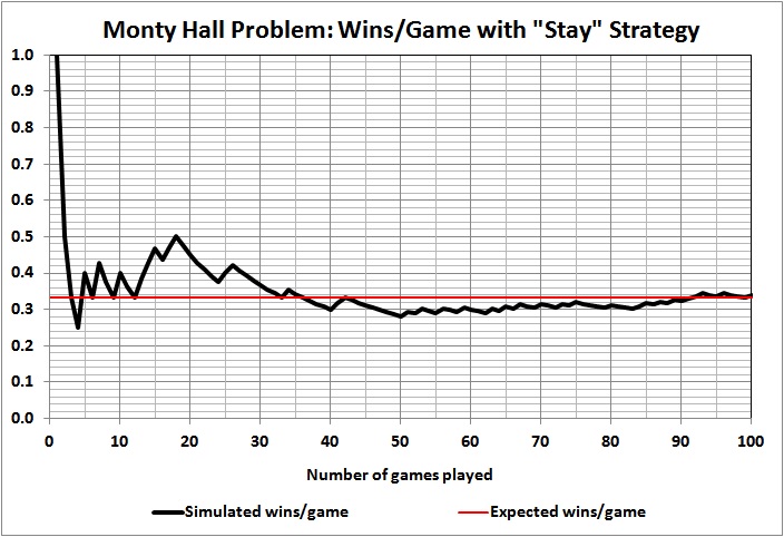
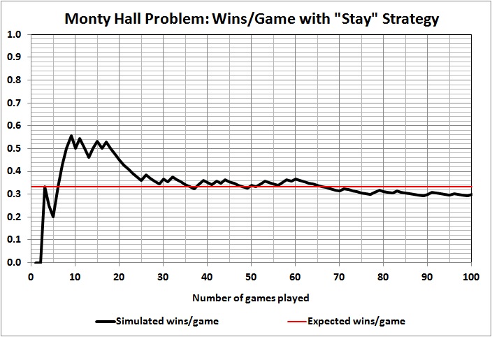
Results of 100 games_1

Results of 100 games_2

Results of 100 games_3

Results of 100 games_4

Results of 100 games_5

Some observations:

Outcomes of individual games are unpredictable, as evidenced by the wild swings and jagged lines, the latter of which persist even at 100 games.

Taking the first game as a proxy for a single-game run of the show, we see that the contestant won that game in just one of the five simulations. To put it another way, in four of the five cases the producer would have thrown away his money on a rapidly depreciating asset (a car) if had offered a car as the prize.

Results vary widely and wildly after the first game. At 10 and 20 games, contestants are doing better than expected in four of the five simulations. At 30 games, contestants are doing as well or better than expected in all five simulations. At 100 games, contestants are doing better than expected in two simulation, worse than expected in two simulation, and exactly as expected in one simulation. What should the producer do with such information? Well, it’s up to the producer and his tolerance for risk. But a prudent producer wouldn’t budget 33 cars or $990,000 just because that’s the expected value of 100 games.

It can take a lot of games to yield an outcome that comes close to 1/3 car per game. A game-show producer could easily lose his shirt by “betting” on 1/3 car per game for a season much shorter than 100 games, and even for a season of 100 games.

*     *     *

The reader’s second additional comment pertains to this exchange:

On what basis other than an understanding of probability would you be optimistic at the prospect of being offered one chance of picking a single Golden Ball worth $1m from a bag of just three balls and pessimistic about your prospects of picking the sole Golden Ball from a barrel of 10,000 balls?

The only difference between the two games is that on the one hand you have a decent (33%) chance of winning and on the other hand you have a lousy (0.01%) chance. Isn’t it these disparate probabilities that give you cause for optimism or pessimism, as the case may be?

“Optimism” and “pessimism” — like “comfort” — are subjective terms for ill-defined states of mind. There are persons who will be “optimistic” about a given situation, and persons who will be “pessimistic” about the same situation. For example: There are hundreds of millions of persons who are “optimistic” about winning various lotteries, even though they know that the grand prize in each lottery will be assigned to only one of millions of possible numbers. By the same token, there are hundreds of millions of persons who, knowing the same facts, refuse to buy lottery tickets because they are “pessimistic” about the likely outcome of doing so. But “optimism” and “pessimism” — like “comfort” — have nothing to do with probability, which isn’t an attribute of a single game.

The reader now says this:

Optimism or pessimism are states as much as something being hot or cold, or a person perspiring or not, and one would find a lot more confidence among contestants playing a single instance of a 1-in-3 game than one would find amongst contestants playing a 1-in-1b game.

Apart from differing probabilities, how would you explain the higher levels of confidence among players of the 1-in-3 game?

Alternatively, what about a “game” involving 2 electrical wires, one live and one neutral, and a game involving one billion electrical wires, only one of which is live?  Contestants are offered $1m if they are prepared to touch one wire.  No one accepts the dare in the 1-in-2 game but a reasonable percentage accept the dare in the 1-in-1b game.

Is the probable outcome of a single event a factor in the different rates of uptake between the two games?

The reader begs the question by introducing “hot or cold” and “perspiring or not,” which have nothing to do with objective probabilities (long-run frequencies of occurrence) and everything to do with individual attitudes toward risk-taking. That was the point of my original response, and I stand by it. The reader simply tries to evade the point by reading the minds of his hypothetical contestants (“higher levels of confidence among players of the 1-in-3 game”). He fails to address the basic issue, which is whether or not there are single-case probabilities — an issue that I addressed at length in “Some Thoughts…”.

The alternative hypotheticals involving electrical wires are just variants of the original one. They add nothing to the discussion.

*     *     *

Enough of this. If the reader — or anyone else — has some good arguments to make in favor of single-case probabilities, drop me a line. If your thoughts have merit, I may write about them.

Signature

The Compleat Monty Hall Problem

Wherein your humble blogger gets to the bottom of the Monty Hall problem, sorts out the conflicting solutions, and declares that the standard solution is the right solution, but not to the Monty Hall problem as it’s usually posed.

THE MONTY HALL PROBLEM AND THE TWO “SOLUTIONS”

The Monty Hall problem, first posed as a statistical puzzle in 1975, has been notorious since 1990, when Marilyn vos Savant wrote about it in Parade. Her solution to the problem, to which I will come, touched off a controversy that has yet to die down. But her solution is now widely accepted as the correct one; I refer to it here as the standard solution.

This is from the Wikipedia entry for the Monty Hall problem:

The Monty Hall problem is a brain teaser, in the form of a probability puzzle (Gruber, Krauss and others), loosely based on the American television game show Let’s Make a Deal and named after its original host, Monty Hall. The problem was originally posed in a letter by Steve Selvin to the American Statistician in 1975 (Selvin 1975a), (Selvin 1975b). It became famous as a question from a reader’s letter quoted in Marilyn vos Savant‘s “Ask Marilyn” column in Parade magazine in 1990 (vos Savant 1990a):

Suppose you’re on a game show, and you’re given the choice of three doors: Behind one door is a car; behind the others, goats. You pick a door, say No. 1, and the host, who knows what’s behind the doors, opens another door, say No. 3, which has a goat. He then says to you, “Do you want to pick door No. 2?” Is it to your advantage to switch your choice?

Here’s a complete statement of the problem:

1. A contestant sees three doors. Behind one of the doors is a valuable prize, which I’ll denote as $. Undesirable or worthless items are behind the other two doors; I’ll denote those items as x.

2. The contestant doesn’t know which door conceals $ and which doors conceal x.

3. The contestant chooses a door at random.

4. The host, who knows what’s behind each of the doors, opens one of the doors not chosen by the contestant.

5. The door chosen by the host may not conceal $; it must conceal an x. That is, the host always opens a door to reveal an x.

6. The host then asks the contestant if he wishes to stay with the door he chose initially (“stay”) or switch to the other unopened door (“switch”).

7. The contestant decides whether to stay or switch.

8. The host then opens the door finally chosen by the contestant.

9. If $ is revealed, the contestant wins; if x is revealed the contestant loses.

One solution (the standard solution) is to switch doors because there’s a 2/3 probability that $ is hidden behind the unopened door that the contestant didn’t choose initially. In vos Savant’s own words:

Yes; you [the contestant] should switch. The first [initially chosen] door has a 1/3 chance of winning, but the second [other unopened] door has a 2/3 chance.

The other solution (the alternative solution) is indifference. Those who propound this solution maintain that there’s a equal chance of finding $ behind either of the doors that remain unopened after the host has opened a door.

As it turns out, the standard solution doesn’t tell a contestant what to do in a particular game. But the standard solution does point to the right strategy for someone who plays or bets on a large number of games.

The alternative solution accurately captures the unpredictability of any particular game. But indifference is only a break-even strategy for a person who plays or bets on a large number of games.

EXPLANATION OF THE STANDARD SOLUTION

The contestant may choose among three doors, and there are three possible ways of arranging the items behind the doors: S x x; x $ x; and x x $. The result is nine possible ways in which a game may unfold:

Equally likely outcomes

Events 1, 5, and 9 each have two branches. But those branches don’t count as separate events. They’re simply subsets of the same event; when the contestant chooses a door that hides $, the host must choose between the two doors that hide x, but he can’t open both of them. And his choice doesn’t affect the outcome of the event.

It’s evident that switching would pay off with a win in 2/3 of the possible events; whereas, staying with the original choice would off in only 1/3 of the possible events. The fractions 1/3 and 2/3 are usually referred to as probabilities: a 2/3 probability of winning $ by switching doors, as against a 1/3 probability of winning $ by staying with the initially chosen door.

Accordingly, proponents of the standard solution — who are now legion — advise the individual (theoretical) contestant to switch. The idea is that switching increases one’s chance (probability) of winning.

A CLOSER LOOK AT THE STANDARD SOLUTION

There are three problems with the standard solution:

1. It incorporates a subtle shift in perspective. The Monty Hall problem, as posed, asks what a contestant should do. The standard solution, on the other hand, represents the expected (long-run average) outcome of many events, that is, many plays of the game. For reasons I’ll come to, the outcome of a single game can’t be described by a probability.

2.  Lists of possibilities, such as those in the diagram above, fail to reflect the randomness inherent in real events.

3. Probabilities emerge from many repetitions of the kinds of events listed above. It is meaningless to ascribe a probability to a single event. In case of the Monty Hall problem, many repetitions of the game will yield probabilities approximating those given in the standard solution, but the outcome of each repetition will be unpredictable. It is therefore meaningless to say that a contestant has a 2/3 chance of winning a game if he switches. A 2/3 chance of winning refers to the expected outcome of many repetitions, where the contestant chooses to switch every time. To put it baldly: How does a person win 2/3 of a game? He either wins or doesn’t win.

Regarding points 2 and 3, I turn to Probability, Statistics and Truth (second revised English edition, 1957), by Richard von Mises:

The rational concept of probability, which is the only basis of probability calculus, applies only to problems in which either the same event repeats itself again and again, or a great number of uniform elements are involved at the same time. Using the language of physics, we may say that in order to apply toe theory of probability we must have a practically unlimited sequence of uniform observations. (p. 11)

*     *     *

In games of dice, the individual event is a single throw of the dice from the box and the attribute is the observation of the number of points shown by the dice. In the same of “heads or tails”, each toss of the coin is an individual event, and the side of the coin which is uppermost is the attribute. (p. 11)

*     *     *

We must now introduce a new term…. This term is “the collective”, and it denotes a sequence of uniform events or processes which differ by certain observable attributes…. All the throws of dice made in the course of a game [of many throws] from a collective wherein the attribute of the single event is the number of points thrown…. The definition of probability which we shall give is concerned with ‘the probability of encountering a single attribute [e.g., winning $ rather than x ] in a given collective [a series of attempts to win $ rather than x ]. (pp. 11-12)

*     *     *

[A] collective is a mass phenomenon or a repetitive event, or, simply, a long sequence of observations for which there are sufficient reasons to believe that the relative frequency of the observed attributed would tend to a fixed limit if the observations were indefinitely continued. The limit will be called the probability of the attribute considered within the collective [emphasis in the original]. (p. 15)

*     *     *

The result of each calculation … is always … nothing else but a probability, or, using our general definition, the relative frequency of a certain event in a sufficiently long (theoretically, infinitely long) sequence of observations. The theory of probability can never lead to a definite statement concerning a single event. The only question that it can answer is: what is to be expected in the course of a very long sequence of observations? It is important to note that this statement remains valid also if the calculated probability has one of the two extreme values 1 or 0 [emphasis added]. (p. 33)

To bring the point home, here are the results of 50 runs of the Monty Hall problem, where each result represents (i) a random initial choice between Door 1, Door 2, and Door 3; (ii) a random array of $, x, and x behind the three doors; (iii) the opening of a door (other than the one initially chosen) to reveal an x; and (iv) a decision, in every case, to switch from the initially chosen door to the other unopened door:

Results of 50 games

What’s relevant here isn’t the fraction of times that $ appears, which is 3/5 — slightly less than the theoretical value of 2/3.  Just look at the utter randomness of the results. The first three outcomes yield the “expected” ratio of two wins to one loss, though in the real game show the two winners and one loser would have been different persons. The same goes for any sequence, even the final — highly “improbable” (i.e., random) — string of nine straight wins (which would have accrued to nine different contestants). And who knows what would have happened in games 51, 52, etc.

If a person wants to win 2/3 of the time, he must find a game show that allows him to continue playing the game until he has reached his goal. As I’ve found in my simulations, it could take as many as 10, 20, 70, or 300 games before the cumulative fraction of wins per game converges on 2/3.

That’s what it means to win 2/3 of the time. It’s not possible to win a single game 2/3 of the time, which is the “logic” of the standard solution as it’s usually presented.

WHAT ABOUT THE ALTERNATIVE SOLUTION?

The alternative solution doesn’t offer a winning strategy. In this view of the Monty Hall problem, it doesn’t matter which unopened door a contestant chooses. In effect, the contestant is advised to flip a coin.

As discussed above, the outcome of any particular game is unpredictable, so a coin flip will do just as well as any other way of choosing a door. But randomly selecting an unopened door isn’t a good strategy for repeated plays of the game. Over the long run, random selection means winning about 1/2 of all games, as opposed to 2/3 for the “switch” strategy. (To see that the expected probability of winning through random selection approaches 1/2, return to the earlier diagram; there, you’ll see that $ occurs in 9/18 = 1/2 of the possible outcomes for “stay” and “switch” combined.)

Proponents of the alternative solution overlook the importance of the host’s selection of a door to open. His choice isn’t random. Therein lies the secret of the standard solution — as a long-run strategy.

WHY THE STANDARD SOLUTION WORKS IN THE LONG RUN

It’s commonly said by proponents of the standard solution that when the host opens a door, he gives away information that the contestant can use to increase his chance of winning that game. One nonsensical version of this explanation goes like this:

  • There’s a 2/3 probability that $ is behind one of the two doors not chosen initially by the contestant.
  • When the host opens a door to reveal x, that 2/3 “collapses” onto the other door that wasn’t chosen initially. (Ooh … a “collapsing” probability. How exotic. Just like Schrödinger’s cat.)

Of course, the host’s action gives away nothing in the context of a single game, the outcome of which is unpredictable. The host’s action does help in the long run, if you’re in a position to play or bet on a large number of games. Here’s how:

  • The contestant’s initial choice (IC) will be wrong 2/3 of the time. That is, in 2/3 of a large number of games, the $ will be behind one of the other two doors.
  • Because of the rules of the game, the host must open one of those other two doors (HC1 and HC2); he can’t open IC.
  • When IC hides an x (which happens 2/3 of the time), either HC1 and HC2 must conceal the $; the one that doesn’t conceal the $ conceals an x.
  • The rules require the host to open the door that conceals an x.
  • Therefore, about 2/3 of the time the $ will be behind HC1 or HC2, and in those cases it will always be behind the door (HC1 or HC2) that the host doesn’t open.
  • It follows that the contestant, by consistently switching from IC to the remaining unopened door (HC1 or HC2), will win the $ about 2/3 of the time.

The host’s action transforms the probability — the long-run frequency — of choosing the winning door from 1/2 to 2/3. But it does so if and only if the player or bettor always switches from IC to HC1 or HC2 (whichever one remains unopened).

You can visualize the steps outlined above by looking at the earlier diagram of possible outcomes.

That’s all there is. There isn’t any more.

Something from Nothing?

I do not know if Lawrence Krauss typifies scientists in his logical obtuseness, but he certainly exemplifies the breed of so-called scientists who proclaim atheism as a scientific necessity.  According to a review by David Albert of Krauss’s recent book, A Universe from Nothing,

the laws of quantum mechanics have in them the makings of a thoroughly scientific and adamantly secular explanation of why there is something rather than nothing.

Albert’s review, which I have quoted extensively elsewhere, comports with Edward Feser’s analysis:

The bulk of the book is devoted to exploring how the energy present in otherwise empty space, together with the laws of physics, might have given rise to the universe as it exists today. This is at first treated as if it were highly relevant to the question of how the universe might have come from nothing—until Krauss acknowledges toward the end of the book that energy, space, and the laws of physics don’t really count as “nothing” after all. Then it is proposed that the laws of physics alone might do the trick—though these too, as he implicitly allows, don’t really count as “nothing” either.

Bill Vallicella puts it this way:

[N]o one can have any objection to a replacement of the old Leibniz question — Why is there something rather than nothing? … — with a physically tractable question, a question of interest to cosmologists and one amenable to a  physics solution. Unfortunately, in the paragraph above, Krauss provides two different replacement questions while stating, absurdly, that the second is a more succinct version of the first:

K1. How can a physical universe arise from an initial condition in which there are no particles, no space and perhaps no time?

K2. Why is there ‘stuff’ instead of empty space?

These are obviously distinct questions.  To answer the first one would have to provide an account of how the universe originated from nothing physical: no particles, no space, and “perhaps” no time.  The second question would be easier to answer because it presupposes the existence of space and does not demand that empty space be itself explained.

Clearly, the questions are distinct.  But Krauss conflates them. Indeed, he waffles between them, reverting to something like the first question after raising the second.  To ask why there is something physical as opposed to nothing physical is quite different from asking why there is physical “stuff” as opposed to empty space.

Several years ago, I explained the futility of attempting to decide the fundamental question of creation and its cause on scientific grounds:

Consider these three categories of knowledge (which long pre-date their use by Secretary of Defense Donald Rumsfeld): known knowns, know unknowns, and unknown unknowns. Here’s how that trichotomy might be applied to a specific aspect of scientific knowledge, namely, Earth’s rotation about the Sun:

1. Known knowns — Earth rotates about the Sun, in accordance with Einstein’s theory of general relativity.

2. Known unknowns — Earth, Sun, and the space between them comprise myriad quantum phenomena (e.g., matter and its interactions of matter in, on, and above the Earth and Sun; the transmission of light from Sun to Earth). We don’t know whether and how quantum phenomena influence Earth’s rotation about the Sun; that is, whether Einsteinian gravity is a partial explanation of a more complete theory of gravity that has been dubbed quantum gravity.

3. Unknown unknowns — Other things might influence Earth’s rotation about the Sun, but we don’t know what those other things are, if there are any.

For the sake of argument, suppose that scientists were as certain about the origin of the universe in the Big Bang as they are about the fact of Earth’s rotation about the Sun. Then, I would write:

1. Known knowns — The universe was created in the Big Bang, and the universe — in the large — has since been “unfolding” in accordance with Einsteinian relativity.

2. Known unknowns — The Big Bang can be thought of as a meta-quantum event, but we don’t know if that event was a manifestation of quantum gravity. (Nor do we know how quantum gravity might be implicated in the subsequent unfolding of the universe.)

3. Unknown unknowns — Other things might have caused the Big Bang, but we don’t know if there were such things or what those other things were — or are.

Thus — to a scientist qua scientist — God and Creation are unknown unknowns because, as unfalsifiable hypotheses, they lie outside the scope of scientific inquiry. Any scientist who pronounces, one way or the other, on the existence of God and the reality of Creation has — for the moment, at least — ceased to be scientist.

Which is not to say that the question of creation is immune to logical analysis; thus:

To say that the world as we know it is the product of chance — and that it may exist only because it is one of vastly many different (but unobservable) worlds resulting from chance — is merely to state a theoretical possibility. Further, it is a possibility that is beyond empirical proof or disproof; it is on a par with science fiction, not with science.

If the world as we know it — our universe — is not the product of chance, what is it? A reasonable answer is found in another post of mine, “Existence and Creation.” Here is the succinct version:

  1. In the material universe, cause precedes effect.
  2. Accordingly, the material universe cannot be self-made. It must have a “starting point,” but the “starting point” cannot be in or of the material universe.
  3. The existence of the universe therefore implies a separate, uncaused cause.

There is no reasonable basis — and certainly no empirical one — on which to prefer atheism to deism or theism. Strident atheists merely practice a “religion” of their own. They have neither logic nor science nor evidence on their side — and eons of belief against them.

Another blogger once said this about the final sentence of that quotation, which I lifted from another post of mine:

I would have to disagree with the last sentence. The problem is epistemology — how do we know what we know? Atheists, especially ‘scientistic’ atheists, take the position that the modern scientific methodology of observation, measurement, and extrapolation from observation and measurement, is sufficient to detect anything that Really Exists — and that the burden of proof is on those who propose that something Really Exists that cannot be reliably observed and measured; which is of course impossible within that mental framework. They have plenty of logic and science on their side, and their ‘evidence’ is the commonly-accepted maxim that it is impossible to prove a negative.

I agree that the problem of drawing conclusions about creation from science (as opposed to logic) is epistemological. The truth and nature of creation is an “unknown unknown” or, more accurately, an “unknowable unknown.” With regard to such questions, scientists do not have logic and science on their side when they asset that the existence of the universe is possible without a creator, as a matter of science (as Krauss does, for example). Moreover, it is scientists who are trying to prove a negative: that there is neither a creator nor the logical necessity of one.

“Something from nothing” is possible, but only if there is a creator who is not part of the “something” that is the proper subject of scientific exploration and explanation.

Related posts:
Atheism, Religion, and Science
The Limits of Science
Three Perspectives on Life: A Parable
Beware of Irrational Atheism
The Creation Model
The Thing about Science
Evolution and Religion
Words of Caution for Scientific Dogmatists
Science, Evolution, Religion, and Liberty
The Legality of Teaching Intelligent Design
Science, Logic, and God
Capitalism, Liberty, and Christianity
Is “Nothing” Possible?
Debunking “Scientific Objectivity”
Science’s Anti-Scientific Bent
Science, Axioms, and Economics
The Big Bang and Atheism
The Universe . . . Four Possibilities
Einstein, Science, and God
Atheism, Religion, and Science Redux
Pascal’s Wager, Morality, and the State
Evolution as God?
The Greatest Mystery
What Is Truth?
The Improbability of Us
A Digression about Probability and Existence
More about Probability and Existence
Existence and Creation
Probability, Existence, and Creation
The Atheism of the Gaps

Probability, Existence, and Creation

A point that I make in “More about Probability and Existence” is made more eloquently and succinctly by Jacques Maritain:

To attempt to demonstrate that the world can be the effect of chance by beginning with the presupposition of this very possibility is to become the victim of a patent sophism or a gross illusion. In order to have the right to apply the calculus of probabilities to the case of the formation of the world, it would be necessary first to have established that the world can be the effect of chance. (Approaches to God, Macmillan paperback edition, pp. 60-1.)

To say that the world as we know it is the product of chance — and that it may exist only because it is one of vastly many different (but unobservable) worlds resulting from chance — is merely to state a theoretical possibility. Further, it is a possibility that is beyond empirical proof or disproof; it is on a par with science fiction, not with science.

If the world as we know it — our universe — is not the product of chance, what is it? A reasonable answer is found in another post of mine, “Existence and Creation.” Here is the succinct version:

  1. In the material universe, cause precedes effect.
  2. Accordingly, the material universe cannot be self-made. It must have a “starting point,” but the “starting point” cannot be in or of the material universe.
  3. The existence of the universe therefore implies a separate, uncaused cause.

There is no reasonable basis — and certainly no empirical one — on which to prefer atheism to deism or theism. Strident atheists merely practice a “religion” of their own. They have neither logic nor science nor evidence on their side — and eons of belief against them.

UPDATE 01/11/16:

Philosopher Gary Gutting writes:

The idea of a cosmological argument is to move from certain known effects to God as their cause. To construct such an argument, we need a principle of causality: a statement of which sorts of things need causes to explain them. The simplest such principle would be: everything has a cause. But this is too strong a claim, since if everything has a cause, then God will have a cause and so be dependent on something else, which would, therefore, have a better claim to be God. A cosmological argument will work only if we have a causal principle that will not apply to God….

A cosmological argument is an effort to carry the search for an explanation as far as it can go, to see if we can discover not just an explanation of some single thing but an explanation of everything—for, we might say, the world (kosmos in Greek) as a whole. Let’s call this an ultimate explanation. We want, therefore, an argument that will show that God is the ultimate explanation. Perhaps, then, the causal principle we need is that there must be an ultimate explanation (provided by an ultimate cause).

Now, however, we need to think more carefully about what an ultimate explanation would explain. We’ve said it’s an explanation of everything, but just what does this mean? Something that needs explanation is, by definition, not self-explanatory. It needs to be explained by something other than itself. As we’ve seen, if we sought an explanation of literally everything, then there would be nothing available to provide the explanation.

If there is to be an ultimate explanation, then, it must be something that itself requires no explanation but explains everything else. The world that the cosmological argument is trying to explain must not be everything but everything that needs an explanation. But what things require explanation?

One plausible answer is that we must explain those things that do exist but might not exist, things that, to use the traditional technical term, are contingent….

Correspondingly, for the cosmological argument to work, the explanation of everything contingent must be something that is not contingent; namely, something that not only exists but also cannot not exist; it must, that is, be necessary. If it weren’t necessary, it would be contingent and so itself in need of explanation. (Notice that what is necessary is not contingent, and vice versa.) Simply put, the God the cosmological argument wants to prove exists has to be a necessary, not a contingent, being.

Here, then, we move to a still better principle of causality: that every contingent thing requires a cause. But we still need to be careful. Most contingent things can be explained by other contingent things. The world (the totality of contingent things) is a complex explanatory system…. If this makes sense, the cosmological argument can’t get off the ground because, as we’ve seen, its God is a necessary being that’s needed to explain what contingent things can’t….

What does this mean for our effort to construct a cosmological argument? It means that our argument must deny that there is an infinite regress of contingent things that explains everything that needs explaining. Otherwise, there’s no need for a necessary God.

This is a crucial stage in our search for a cosmological argument. We have a plausible principle of causality: any contingent being needs a cause. We now see that we need another premise: that an infinite regress of contingent things cannot explain everything that needs explaining….

We can agree that there might be an infinite series of contingent explainers but still maintain that such an infinite series itself needs an explanation. We might, in effect, grant that there could be an infinite series of tortoises, each supporting the other—and the whole chain supporting the Earth—but still insist that there must be some explanation for why all those tortoises exist. That is, our argument will require that an infinite regress of contingent things must itself have an explanation. This gives us the two key premises of our cosmological argument: a principle of causality and a principle for excluding an infinite regress.

Now we can formulate our argument:

  1. There are contingent beings.
  2. The existence of any contingent being has an explanation.
  3. Such an explanation must be provided by either a necessary being or by an infinite regress of contingent beings.
  4. An explanation by means of an infinite regress of contingent beings is itself in need of an explanation by a necessary being.
  5. Therefore, there is a necessary being that explains the existence of contingent beings.

This argument is logically valid; that is, if the premises are true, then the conclusion is true…. [“Can We Prove That God Exists? Richard Dawkins and the Limits of Faith and Atheism,” Salon, November 29, 2015]

That looks like my argument.

Related posts:
Atheism, Religion, and Science
The Limits of Science
Three Perspectives on Life: A Parable
Beware of Irrational Atheism
The Creation Model
The Thing about Science
Evolution and Religion
Words of Caution for Scientific Dogmatists
Science, Evolution, Religion, and Liberty
The Legality of Teaching Intelligent Design
Science, Logic, and God
Capitalism, Liberty, and Christianity
Is “Nothing” Possible?
Debunking “Scientific Objectivity”
Science’s Anti-Scientific Bent
Science, Axioms, and Economics
The Big Bang and Atheism
The Universe . . . Four Possibilities
Einstein, Science, and God
Atheism, Religion, and Science Redux
Pascal’s Wager, Morality, and the State
Evolution as God?
The Greatest Mystery
What Is Truth?
The Improbability of Us
A Digression about Probability and Existence
More about Probability and Existence
Existence and Creation

More about Probability and Existence

In “A Digression about Probability and Existence” I address

the view that there is life as we know it — an outcome with a low, prior probability given the (theoretical) multitude of possible configurations of the universe — only because there are vastly many actual or possible universes with vastly many configurations.

I observe that

[i]n this view, life as we know it is an improbable phenomenon that we are able to witness only because we happen to exist in one of the multitude of possible or actual universes.

I should have pointed out that it is impossible to know whether life as we know it is a low-probability event. Such a conclusion rests on an unsupportable assumption: the existence of a universe which is “fine tuned” to enable life is a low-probability event. And yet, that assumption is the basis for assertions that the existence of our universe — with its life-supporting combination of matter, energy, and physical laws — “proves” that there must be other universes because ours is so unlikely. Such “logic” is an edifice of rank circularity constructed on a foundation of pure supposition.

Such “logic,” moreover, misapplies the concept “probability.” No object or event has a probability (knowable chance of happening) unless it meets the following conditions:

1. The object or event is a member of a collective of observable phenomena, where every member of the collective has common features.

2. The collective is a mass phenomenon or an unlimited sequence of observations, where (a) the relative frequencies of particular attributes within the collective tend to fixed limits and (b) these fixed limits remain the same for reasonably large subsets of the collective. (Adapted from “Summary of the Definition,” on pp. 28-9 in Chapter 1, “The Definition of Probability,” of Richard von Mises’s Probability, Statistics and Truth, 1957 Dover edition.)

Mises, obviously, was a  “frequentist,” and his view of probability is known as “frequentism.” Despite the criticisms of frequentism (follow the preceding link), it offers the only rigorous view of probability. Nor does it insist (as suggested at the link) that a probability is a precisely knowable or fixed value. But it is a quantifiable value, based on observations of actual objects or events.

Other approaches to probability are vague and subjective. There are, for example, degrees of belief (probabilistic logic), statements of propensity (probabilistic propensity), and “priors” (Bayesian probability). Unlike frequentism, these appeal to speculation, impressions, and preconceptions. Reliance on such notions of probability as evidence of the actual likelihood of an event is the quintessence of circularity.

In summary, there is no sound basis in logic or empirical science for the assertion that the universe we know is a highly improbable one and, therefore must be one of vastly many universes — if it was not the conscious creation of an exogenous force or being (i.e., God). The universe we know simply “is” — and that is all we know or probably can know, as a matter of science.

Related posts:
Atheism, Religion, and Science
The Limits of Science
Three Perspectives on Life: A Parable
Beware of Irrational Atheism
The Creation Model
The Thing about Science
Evolution and Religion
Words of Caution for Scientific Dogmatists
Science, Evolution, Religion, and Liberty
The Legality of Teaching Intelligent Design
Science, Logic, and God
Capitalism, Liberty, and Christianity
Is “Nothing” Possible?
A Dissonant Vision
Debunking “Scientific Objectivity”
Science’s Anti-Scientific Bent
Science, Axioms, and Economics
The Big Bang and Atheism
The Universe . . . Four Possibilities
Einstein, Science, and God
Atheism, Religion, and Science Redux
Pascal’s Wager, Morality, and the State
Evolution as God?
The Greatest Mystery
What Is Truth?
The Improbability of Us
A Digression about Probability and Existence

A Digression about Probability and Existence

The probability of an event can be the probability that it will (or could) happen, or the relative occurrence of the event as that occurrence is observed in nature or experiment.

It is known, for example, that the following prior probabilities attach to the outcome of a single roll of a pair of fair dice:

And if a single person rolled a pair of dice 1,000,000 times or 1,000,000 persons each rolled a pair of dice once, the result would be close (but not necessarily identical) to this:

But the fact that a single player, on a single roll, throws a 2, 5, 9, 12, or any other sum tells us nothing about the number of rolls the player has made or will make, nor does it tell us anything about the number of players who may have rolled dice at the same moment. All it tells us is that the player has attained a particular result on that particular roll of the dice.

This is at odds with the view that there is life as we know it — an outcome with a low, prior probability given the (theoretical) multitude of possible configurations of the universe — only because there are vastly many actual or possible universes with vastly many configurations. In this view, life as we know it is an improbable phenomenon that we are able to witness only because we happen to exist in one of the multitude of possible or actual universes.

So, is our universe and the life that has arisen in it a consequence of design, or is it all a matter of “luck”? And if it is due to “luck,” what created the material of which the universe is made and what determined the laws that are evident in the actions of that material?

Related posts:
Atheism, Religion, and Science
The Limits of Science
Three Perspectives on Life: A Parable
Beware of Irrational Atheism
The Creation Model
The Thing about Science
Evolution and Religion
Words of Caution for Scientific Dogmatists
Science, Evolution, Religion, and Liberty
The Legality of Teaching Intelligent Design
Science, Logic, and God
Capitalism, Liberty, and Christianity
Is “Nothing” Possible?
A Dissonant Vision
Debunking “Scientific Objectivity”
Science’s Anti-Scientific Bent
Science, Axioms, and Economics
The Big Bang and Atheism
The Universe . . . Four Possibilities
Einstein, Science, and God
Atheism, Religion, and Science Redux
Pascal’s Wager, Morality, and the State
Evolution as God?
The Greatest Mystery
What Is Truth?
The Improbability of Us