A labor-supply curve, in economics, is a graphical or mathematical representation of the number of units of labor (work) of a specified kind that will be offered in a specified period of time (hour, day, week, etc.) at various rates of compensation (hourly wage or periodic salary or expected earnings from self-employment, plus the monetary value of benefits such as vacation time, pension contributions, etc.). A supply curve (like a demand curve) is ephemeral, in that it consists of the summation of the supply curves of many persons (or firms), each of which varies widely at a given time and shifts over time.
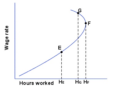
A person’s labor-supply curve is said to represent the choices that the person would make between work and leisure at various rates of compensation. On the assumption that leisure becomes more attractive than work at some point (i.e., a relatively high wage rate or salary that affords the person more than “enough” on which to live), the labor-supply curve is depicted as backward-bending after that point; that is, the worker will work less as his wage rate rises above the critical point. Graphically:
Figure 1
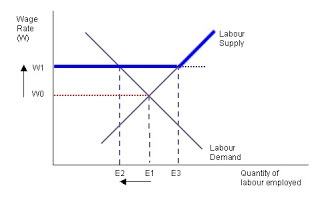
There are also complications due to unionization and minimum wage laws, both of which tend to set a wage rate that is above the wage that most workers would accept in a one-on-one transaction with an employer or prospective employer. (If unions or governments don’t mean to bargain for or dictate a wage above that which an individual worker could obtain on his own, that would vitiate the main justification for unionization and minimum-wage laws.) In any event, the effect of unionization and minimum wage laws is to deprive many workers of employment; thus:
Figure 2

The preceding relationships, interesting as they are, don’t paint a complete picture of the determinants of a person’s labor-supply curve. They are, perforce, inadequate to the task of explaining how various conglomerations of workers (e.g., unskilled laborers in Texas, pipefitters in Michigan, plastic surgeons in Malibu) will respond to compensation incentives.
For one thing, leisure — in the standard treatment — is a catchall for non-work activities: eating, sleeping, recreation, etc. It is simplistic to bundle those disparate activities. For another thing, most workers these days aren’t affected (directly, at least) by unionization or minimum wage laws. In general, the standard treatments fail to account adequately for other factors that may influence a person’s willingness to work for a give rate of compensation; for example, the perceived need to sustain a certain standard of living by working more to offset a reduction in one’s rate of compensation. I therefore submit the following step-by-step analysis of the labor-supply function, which is more complete and accordingly more complex than the standard treatments.
I will begin at the beginning, though I will refer to Figures 1 and 2 where they apply.
A person’s willingness and ability to perform a certain amount of work (L) of a particular kind is a function of several parameters: C, U, B, X, T, N, S, and E, each of which is defined below. I begin with the basic relationship between L and C, and then introduce the variations due to the other parameters.
C = total net compensation for work. This is the product of net compensation per unit of work (c) and the number of units of work (L). Net compensation is the after-tax, discounted present value of wages/salary and benefits (as perceived by the worker), for a given set of government policies that affect net compensation, directly or indirectly. In a simple labor-supply function, L = f(c), in which W responds positively and monotonically to increases in c; that is, the function is represented by an upward-sloping line (L), where c is measured on the vertical axis and L is measured on the horizontal axis:
Figure 3

(The rectangle bounded by the horizontal and vertical axes and the dashed lines that represent specific numbers of units of work, L1, and net compensation per unit, c1, has an area equal to the total compensation for that combination of c and L, which in this case is C1.)
U = utility or satisfaction derived from consumption and wealth accumulation resulting from work. This is usually depicted as a positive and rising relationship of the kind shown in the preceding graph. That is to say, the standard labor-supply curve is upward-rising because U generally increases as c rises (that is, as L rises) because of improvements in the quantity and quality of goods consumed and the accumulation of wealth (which provides even more access to goods of high quality, greater social standing, etc.). The following parameters complicate this seemingly simple relationship between c and L.
B = the effect of meeting basic necessities on the amount of labor that a worker is willing to offer. One factor that complicates a worker’s labor-supply function is the need to earn enough to cover basic necessities (e.g., minimal food, clothing, and shelter). The worker may be willing to work as much as required to pay for those necessities. For example, if his necessities cost him $100 a week and he can earn $10 an hour, he will be willing to work at least 10 hours a week, but if he can earn only $5 an hour, he will have to work at least 20 hours a week to pay for his basic necessities. It is entirely possible that a person who earns $500,000 a year will consider that amount necessary to meet his basic necessities, and that a change in his earning power or government policies will induce him to work more in order to net $500,000 a year. In any event, here is a depiction of the relevant portion of a labor-supply curve where B prevails:
Figure 4

If the worker is willing and able to deliver his labor beyond L3, his supply function would extend upward and to the right from that point. That is, having satisfied his basic needs, he would then be able to increase his utility by working more hours for higher rates of compensation.
X = the effect of changes in government policies on net compensation per unit of work, and therefore on the number of units of work that a worker will offer at a given rate of net compensation. If a worker has certain basic necessities (e.g., minimal food, clothing, and shelter), he will offer to work at least as much as required to meet those necessities, and may therefore offer to increase the number of units worked in response to X. For example, if the necessities have a cost to him $500 per week, he will offer to work as many hours as necessary to earn net compensation of $500 per week. And if his taxes increase by, say, $50 per week, he will seek additional work in order to offset the tax increase. But, if he is earning more than is required to cover his basic necessities, a tax increase of $50 a week — an effective reduction in his compensation — will cause him to work less.
In this case, the graph of the relevant portion of the worker’s supply curve would look like Figure 3 or Figure 4, but c would be higher at each point along L; that is, the new supply curve would be above and parallel to the old supply curve.
T = taste for work of a particular kind. T is positive and rising with L if the work itself offers some pleasure to the worker (e.g., a doctor who enjoys helping the sick, an athlete who enjoys his sport for its own sake, a lawyer who revels in argumentation), or negative and declining with L if the worker works only for the compensation because of his distaste for the work (e.g., cleaning toilets, babysitting brats, working for pointy-haired bosses). This “psychic income” or “psychic penalty” raises or lowers the amount of work that the worker is willing to perform for a given rate of compensation (c).
Imagine a person who is capable of performing two different kinds of labor, X and Y. If Figure 3 or Figure 4 refers to X, and if the person has a “taste” for Y, his supply curve will for Y lie below the ones depicted in Figure 3 and 4; that is, he will require less compensation to do Y rather than X.
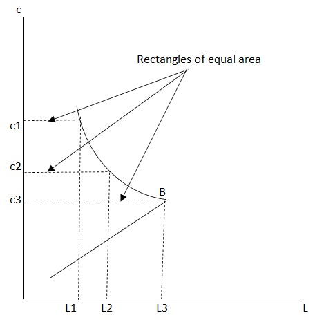
N = preference for non-work time (which includes leisure and time spent on personal functions such as meeting familial obligations, eating, and sleeping). This is the backward-bending relationship depicted in Figure 1. The portion of the supply curve that runs upward and to the right incorporates the tradeoff between compensation and leisure. But at some threshold value of C, the worker responds to higher c by reducing L. It seems to me that this effect should be depicted in this way:
Figure 5

That is, the worker reaches his “saturation” point at L3 and reduces the amount of work that he does as c rises past c3. In this case, he reduces his work time so that his total compensation remains the same as it was at L3.
S = subsidies that discourage work (e.g., unemployment benefits, “disability” payments, food stamps, subsidized housing). Where these are available to a worker, they reduce the amount of work that he is willing to do because they enable him to attain a given U without working. T may be positive and offsetting, but this is unlikely among workers who qualify for subsidies. The S effect pushes the supply curve upward; that is, less labor is offered for a given rate of compensation.
E = external forces that limit the amount of labor that a person is able to offer. There are at least two significant forces of this kind. One is the effect of laws and regulations that dictate the maximum amount of work that may be performed (e.g., zero in the case of most children under the age of 16) or the rate of compensation that must be paid (e.g., the minimum wage, overtime pay for persons in certain occupations). The other major force is the effect of employer-union contracts that dictate rates of compensation and hours of work that cannot possibly reflect the uncoerced preferences of many (or most) individual workers. (E, in its various manifestations, is treated in standard economics by overlaying “floors” or “ceilings” on the labor-supply curve.)
Figure 2 depicts this effect.
In conclusion, a labor-supply curve — even that of one person — can be a complex function, and one that responds in various ways to parameters other than the utility that is gained (or lost) by working more (or less). It is hard to imagine that a meaningful supply curve can be drawn for whole classes of workers. To draw such a curve, the workers must be rather homogeneous in their skills, their tastes (for leisure and other things), their wealth (which can strongly influence one’s willingness to perform certain kinds of work), and their exposure to various governmental policies (unionization, minimum wage laws, etc.). The fluidity of the labor market in the age of the “gig economy” supports my view.