The Minimum Wage Revisited

Posted on October 13, 2021 by Loquitur Veritatem

A post by Arnold Kling (askblog) reminds me of a post of mine from 2009. Kling begins noting the Nobel prize that was awarded to David Card and two others. It was Card and his late collaborator, Alan Krueger, who “proved” that the minimum wage doesn’t cause unemployment.

Kling notes that

Noah Smith goes way overboard in praise of the new laureates. He makes it sound as though the results that David Card and Alan Krueger claimed about the minimum wage were only controversial because they were surprising. But they were also controversial because they were wrong.

Here is the abstract of the paper to which the second link in the block quotation leads:

We re-evaluate the evidence from Card and Krueger’s (1994) New Jersey-Pennsylvania minimum wage experiment, using new data based on actual payroll records from 230 Burger King, KFC, Wendy’s, and Roy Rogers restaurants in New Jersey and Pennsylvania. We compare results using these payroll data to those using CK’s data, which were collected by telephone surveys. We have two findings to report. First, the data collected by CK appear to indicate greater employment variation over the eight-month period between their surveys than do the payroll data. For example, in the full sample the standard deviation of employment change in CK’s data is three times as large as that in the payroll data. Second, estimates of the employment effect of the New Jersey minimum wage increase from the payroll data lead to the opposite conclusion from that reached by CK. For comparable sets of restaurants, differences-in-differences estimates using CK’s data imply that the New Jersey minimum wage increase (of 18.8 percent) resulted in an employment increase of 17.6 percent relative to the Pennsylvania control group, an elasticity of 0.93. In contrast, estimates based on the payroll data suggest that the New Jersey minimum wage increase led to a 4.6 percent decrease in employment in New Jersey relative to the Pennsylvania control group. This decrease is statistically significant at the five-percent level and implies an elasticity of employment with respect to the minimum wage of -0.24.

That’s far from the only time that Card and Krueger’s “proof” has been demolished.

I joined the bandwagon in 2009, with an analysis documented in this post, which ends thus:

On the basis of the robust results [derived from data for 1959 – 2009,] I draw the following conclusions:

The baseline unemployment rate for 16-19 YO [year-olds] is about 9 percent.

Unemployment around the baseline changes by about 1.5 percentage points for every percentage-point change in the unemployment rate for 20+ YO.

The minimum wage, when effective, raises the unemployment rate for 16-19 YO by 0.6 percentage points.

Therefore, given the current number of 16 to 19 year old males in the labor force (about 3.3 million), some 20,000 will lose or fail to find jobs because of yesterday’s boost in the minimum wage. Yes, 20,000 is a small fraction of 3.3 million (0.6 percent), but it is a real, heartbreaking number — 20,000 young men for whom almost any hourly wage would be a blessing.

But the “bleeding hearts” who insist on setting a minimum wage, and raising it periodically, don’t care about those 20,000 young men — they only care about their cheaply won reputation for “compassion.”

The minimum wage is just another blow to liberty and prosperity from the left, which holds that Americans must be impoverished to battle the chimera of anthropogenic global warming, that police (who protect the poor as well as the rich) must be defunded, that people should be paid not to work, that the expression of views contrary to leftist dogma is criminal, and that human life may be disposed of like garbage.

Unorthodox Economics: 4. A Parable of Political Economy

Posted on February 24, 2017 by Loquitur Veritatem

This is the fourth entry in what I hope will become a book-length series of posts. That result, if it comes to pass, will amount to an unorthodox economics textbook. This first chapter gives a hint of things to come. Here are the chapters that have been posted to date:

1. What Is Economics?
2. Pitfalls
3. What Is Scientific about Economics?
4. A Parable of Political Economy
5. Economic Progress, Microeconomics, and Macroeconomics

Imagine a simple society in which Jack and Jill own neighboring farms that are equally endowed in natural resources, tools, and equipment. Jack makes bread and Jill makes butter. Jack also could make butter and Jill also could make bread, but both of them have learned that they are better off if they specialize. Thus:

Jack can make 1 loaf of bread or 0.5 pound of butter a day. (The rate of transformation is linear; e.g. Jack could make 0.5 loaf of bread and 0.25 pound of butter daily.)

Jill can make 1 loaf of bread or 1 pound of butter a day. (Again, the rate of transformation is linear; Jill could make 0.5 loaf of bread and 0.5 pound of butter daily.)

If both Jack and Jill make bread and butter their total daily output might be 1 loaf and 0.75 pounds.

Alternatively, if Jack specializes in bread and Jill specializes in butter their total daily output could be 1 loaf and 1 pound.

Jill is more intelligent than Jack, and thus more innovative. That’s why she is able to reap as much wheat and make as much bread as Jack, even though he’s stronger. That’s also why she’s able to produce twice as much butter as Jack.

Jill has an absolute advantage over Jack, in that she can make as much bread as he can, and more butter than he can. But Jack has a comparative advantage in the production of bread; if he specializes in bread and Jill specializes in butter, he and Jill will be better off than if they both produce bread and butter for themselves.

Jack and Jill negotiate the exchange rate between bread and butter. Each ends up with 0.5 loaf of bread; but Jill gets 0.6 pound of butter to Jack’s 0.4 pound. Jill ends up with more butter than Jack because her greater productivity puts in her in superior bargaining position. In sum, she earns more because she produces more.

Jack and Jill have another neighbor, June, who makes clothing. Jack and Jill are more productive when they’re properly clothed during the colder months of the year. So they’re willing to trade some of their output to June, in return for heavy clothing.

Jerry, another neighbor, is a laborer who used to work for Jack and Jill, but has been unemployed for a long time because of Jill’s technological innovations. Jerry barely subsists on the fruit and game that he’s able to find and catch. Jack and Jill would hire Jerry but he insists on a wage that they can’t afford to pay unless they spends less to maintain their equipment, which would eventually result in a lower rate of output.

Along comes Juan, a wanderer from another region, who has nothing to offer but his labor. Juan is willing to work for a lower wage than Jerry, but has to be fed and clothed so that he becomes strong enough to deliver the requisite amount of labor to be worthy of hire.

Jack, Jill, and June meet to discuss Jerry and Juan. They are worried about Jerry because he’s a neighbor whom they’ve known for a long time. They also empathize with Juan’s plight, though they’re not attached to him because he’s a stranger and doesn’t speak their language well.

Jake — the gunslinger hired by Jack, Jill, and June to protect them from marauders — invites himself the meeting and brings Jerry with him. Jake likes to offset his stern image by feigning compassion. He tells Jack and Jill that they have a duty to pay Jerry the wage that he demands. He also requires Jack and Jill to feed and clothe Juan until he’s ready to work, and then they must hire him and pay him the same wage as Jerry. Jack and Jill demur because they can’t afford to do what Jake demands and make enough bread and butter to sustain their families and put something aside for retirement. June, who reacts with great sympathy to every misfortune around her — perceived and real — sides with Jake. Jerry argues that he should be helped, but Juan shouldn’t be helped because he’s just a stranger with a strange accent who’s looking for a handout.

Jake the gunslinger, disregarding Jerry’s reservation about Juan, announces that Jack and Jill must abide by his decision, inasmuch as there are 3 votes for it and only 2 votes against it — and he has the gun.

What happens next? Several things:

Jack and Jill quite properly accuse Jake of breach of contract. He has assumed a power that wasn’t given to him by Jack, Jill, and June when they hired him. Jake merely laughs at them.

Jack, Jill, and June (though she doesn’t understand it) have lost control of their businesses. They can no longer produce their goods efficiently. This means less output, that is less to trade with each other. Less output also means that they won’t be able to invest as much as before in the improvement and expansion of their operations.

June is happy, for the moment, because Jake sided with her. But she will be unhappy when Jake abuses his authority in a way that she disapproves, and when she finally understands what Jake has done to her business.

Jack and Jill have good reason to resent Juan and Jerry for using Jake to coerce them, and June for siding with Jerry and Juan. There is now a rift that will hinder cooperation for mutual benefit (e.g., willingness to help each other in times of illness).

Juan and Jerry have become dependent on Jake, thus undermining their ability to develop marketable skills and good work habits. Their dependency will keep them mired in near-poverty.

In a sane world, Jack and Jill would get rid of Jake, and the others would applaud them for doing it.

* * *

Say’s Law, Government, and Unemployment

Posted on September 16, 2011 by Loquitur Veritatem

“Supply creates its own demand,” or so goes the popular interpretation of Say’s law. (More about that, below.) But if what you have on offer is not in demand by others, you are out of luck.

That is the point of Megan McArdle’s post, “The New New New Economy.” McArdle writes:

One of my first jobs out of school, way back in 1994, was as a secretary. I’d be shocked to find that any of the executives at that organization still have secretaries–maybe the executive director, but maybe not even him. Already at the time there wasn’t really enough for me to do; my boss had a secretary because, well, people in his position did. That’s not because the work was being outsourced to Bangalore, but because computers and the internet were eliminating much of the coolie labor that secretaries used to take care of. And of course, the recession is accelerating the pace of change–and leaving the people who are displaced fewer options to transition.

Government interventions that destroy jobs — the minimum wage, capital gains taxes, progressive taxation, etc. — exacerbate the problem because they prevent low-skilled workers (teenagers, mainly) from stepping onto the bottom rung of the employment ladder and eventually acquiring skills (or the money with which to acquire skills) that enable them to compete in an increasingly cyber-mated economy.

Which brings me back to Say’s law, explained succinctly by Steven Horwitz in “Understanding Say’s Law of Markets“:

Say was making the claim that production is the source of demand. One’s ability to demand goods and services from others derives from the income produced by one’s own acts of production. Wealth is created by production not by consumption. My ability to demand food, clothing, and shelter derives from the productivity of my labor or my nonlabor assets. The higher (lower) that productivity, the higher (lower) is my power to demand.

When a firm adopts a more productive technology — one that enables it to reduce the price of a product or service and/or offer a better product or service for the same price — the firm benefits and its customers and potential customers benefit. The firm can reap higher profits (if it is in a competitive position to do so) by “sharing” the productivity gains with customers through its pricing strategy. Customers and potential customers, by the same token reap the benefit of a better and/or less expensive product or service.

Who is made worse off? The workers whose skills are such that they cannot produce things that are valued by consumers. Or, if they can produce them, they cannot produce them as cheaply as, say, an automated system. And that system may well have been introduced because government policies of the kind mentioned above make it less profitable for firms to employ labor.

Whose “fault” is that? In a free-market economy, it would be no one’s fault; it would be what it is: an unfortunate subset of the populace lacking the wherewithal to produce what others want. It follows that governmental interventions have created a large (and growing) additional subset of the populace who could — and should — blame their fate upon the minimum wage; capital gains taxes; progressive taxation; regulations that restrict inputs, processes, and outputs; and all other government policies that discourage employment, saving, capital formation, and business expansion.

Does the Minimum Wage Increase Unemployment?

Posted on July 25, 2009 by Loquitur Veritatem

Yes!

I have not a shred of doubt that the minimum wage increases unemployment, especially among the most vulnerable group of workers: males aged 16 to 19.

Anyone who claims that the minimum wage does not affect unemployment among that vulnerable group is guilty of (a) ingesting a controlled substance, (b) wishing upon a star, or — most likely — (c) indulging in a mindless display of vicarious “compassion.”

Economists have waged a spirited mini-war over the minimum-wage issue, to no conclusive end. But anyone who tells you that a wage increase that is forced on businesses by government will not lead to a rise in unemployment is one of three things: an economist with an agenda, a politician with an agenda, a person who has never run a business. There is considerable overlap among the three categories.

I have run a business, and I have worked for the minimum wage (and less). On behalf of business owners and young male workers, I am here to protest further increases in the minimum wage. My protest is entirely evidence-based — no marching, shouting, or singing for me. Facts are my friends, even if they are inimical to Left-wing economists, politicians, and other members of the reality-challenged camp.

I begin with time series on unemployment among males — ages 16 to 19 and 20 and older — for the period January 1948 through June 2009. (These time series are available via this page on the BLS website.) If it is true that the minimum wage targets younger males, the unemployment rate for 16 to 19 year-old males (16-19 YO) will rise faster or decrease less quickly than the unemployment rate for 20+ year-old males (20+ YO) whenever the minimum wage is increased. The precise change will depend on such factors as the propensity of young males to attend college — which has risen over time — and the value of the minimum wage in relation to prevailing wage rates for the industries which typically employ low-skilled workers. But those factors should have little influence on observed month-to-month changes in unemployment rates.

I use two methods to estimate the effects of minimum wage on the unemployment rate of 16-19 YO: graphical analysis and linear regression.

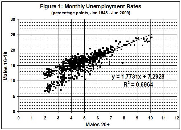
I begin by finding the long-term relationship between the unemployment rates for 16-19 YO and 20+ YO. As it turns out, there is a statistical artifact in the unemployment data, an artifact that is unexplained by this BLS document, which outlines changes in methods of data collection and analysis over the years. The relationship between the two time series is stable through March 1959, when it shifts abruptly. The markedness of the shift can be seen in the contrast between figure 1, which covers the entire period, and figures 2 and 3, which subdivide the entire period into two sub-periods.

090725_Minimum wage and unemployment_fig 1

090725_Minimum wage and unemployment_fig 2

090725_Minimum wage and unemployment_fig 3

For the graphical analysis, I use the equations shown in figures 2 and 3 to determine a baseline relationship between the unemployment rate for 20+ YO (“x”) and the unemployment rate for 16-19 YO (“y”). The equation in figure 2 yields a baseline unemployment rate for 16-19 YO for each month from January 1948 through March 1959; the equation in figure 3, a baseline unemployment rate for 16-19 YO for each month from April 1959 through June 2009. Combining the results, I obtain a baseline estimate for the entire period, January 1948 through June 2009.

I then find, for each month, a residual value for unemployment among 16-19 YO. The residual (actual value minus baseline estimate) is positive when unemployment among 16-19 YO is higher than expected, and negative when 16-19 YO unemployment is lower than expected. Again, this is unemployment of 16-19 YO relative to 20+ YO. Given the stable baseline relationships between the two unemployment rates (when the time series are subdivided as described above), the values of the residuals (month-to-month deviations from the baseline) can reasonably be attributed to changes in the minimum wage.

For purposes of my analysis, I adopt the following conventions:

A change in the minimum wage begins to affect unemployment among 16-19 YO in the month it becomes law, when the legally effective date falls near the start of the month. A change becomes effective in the month following its legally effective date when that date falls near the end of the month. (All of the effective dates have thus far been on the 1st, 3rd, 24th, and 25th of a month.)

In either event, the change in the minimum wage affects unemployment among 16-19 YO for 6 months, including the month in which it becomes effective, as reckoned above.

In other words, I assume that employers (by and large) do not anticipate the minimum wage and begin to fire employees before the effective date of an increase. I assume, rather, that employers (by and large) respond to the minimum wage by failing to hire 16-19 YO who are new to the labor force. Finally, I assume that the non-hiring effect lasts about 6 months — in which time prevailing wage rates for 16-19 YO move toward toward (and perhaps exceed) the minimum wage, thus eventually blunting the effect of the minimum wage on unemployment.

I relax the 6-month rule during eras when the minimum wage rises annually, or nearly so. I assume that during such eras employers anticipate scheduled increases in the minimum wage by continuously suppressing their demand for 16-19 YO labor. (There are four such eras: the first runs from September 1963 through July 1971; the second, from May 1974 through June 1981; the third, from May 1996 through February 1998; the fourth, from July 2007 to the present, and presumably beyond.)

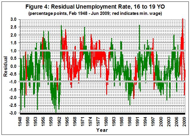
With that prelude, I present the following graph of the relationship between residual unemployment among 16-19 YO and the effective periods of minimum wage increases.

090725_Minimum wage and unemployment_fig 4

The jagged, green and red line represents the residual unemployment rate for 16-19 YO. The green portions of the line denote periods in which the minimum wage is ineffective; the red portions of the line denote periods in which the minimum wage is effective. The horizontal gray bands at +1 and -1 denote the normal range of the residuals, one standard deviation above and below the mean, which is zero.

It is obvious that higher residuals (greater unemployment) are generally associated with periods in which the minimum wage is effective; that is, most portions of the line that lie above the normal range are red. Conversely, lower residuals (less unemployment) are generally associated with periods in which the minimum wage is ineffective; that is, most portions of the line that lie below the normal range are green. (Similar results obtain for variations in which employers anticipate the minimum wage increase, for example, by firing or reduced hiring in the preceding 3 months, while the increase affects employment for only 3 months after it becomes law.)

Having shown that there is an obvious relationship between 16-19 YO unemployment and the minimum wage, I now quantify it. Because of the distinctly different relationships between 16-19 YO unemployment and 20+ YO unemployment in the two sub-periods (January 1948 – March 1959, April 1959 – June 2009), I estimate a separate regression equation for each sub-period.

For the first sub-period, I find the following relationship:

Unemployment rate for 16-19 YO (in percentage points) = 3.913 + 1.828 x unemployment rate for 20+ YO + 0.501 x dummy variable for minimum wage (1 if in effect, 0 if not)

Adjusted R-squared: 0.858; standard error of the estimate: 9 percent of the mean value of 16-19 YO unemployment rate; t-statistics on the intercept and coefficients: 14.663, 28.222, 1.635.

Here is the result for the second sub-period:

Unemployment rate for 16-19 YO (in percentage points) = 8.940 + 1.528 x unemployment rate for 20+ YO + 0.610 x dummy variable for minimum wage (1 if in effect, 0 if not)

Adjusted R-squared: 0.855; standard error of the estimate: 6 percent of the mean value of 16-19 YO unemployment rate; t-statistics on the intercept and coefficients: 62.592, 59.289, 7.495.

On the basis of the robust results for the second sub-period, which is much longer and current, I draw the following conclusions:

The baseline unemployment rate for 16-19 YO is about 9 percent.

Unemployment around the baseline changes by about 1.5 percentage points for every percentage-point change in the unemployment rate for 20+ YO.

The minimum wage, when effective, raises the unemployment rate for 16-19 YO by 0.6 percentage points.

Therefore, given the current number of 16 to 19 year old males in the labor force (about 3.3 million), some 20,000 will lose or fail to find jobs because of yesterday’s boost in the minimum wage. Yes, 20,000 is a small fraction of 3.3 million (0.6 percent), but it is a real, heartbreaking number — 20,000 young men for whom almost any hourly wage would be a blessing.

But the “bleeding hearts” who insist on setting a minimum wage, and raising it periodically, don’t care about those 20,000 young men — they only care about their cheaply won reputation for “compassion.”

UPDATE (09/08/09):

A relevant post by Don Boudreaux:

Here’s a second letter that I sent today to the New York Times:

Gary Chaison misses the real, if unintended, lesson of the Russell Sage Foundation study that finds that low-skilled workers routinely keep working for employers who violate statutory employment regulations such as the minimum-wage (Letters, September 8). This real lesson is that economists’ conventional wisdom about the negative consequences of the minimum-wage likely is true after all.

Fifteen years ago, David Card and Alan Krueger made headlines by purporting to show that a higher minimum-wage, contrary to economists’ conventional wisdom, doesn’t reduce employment of low-skilled workers. The RSF study casts significant doubt on Card-Krueger. First, because the minimum-wage itself is circumvented in practice, its negative effect on employment is muted, perhaps to the point of becoming statistically imperceptible. Second, employers’ and employees’ success at evading other employment regulations – such as mandatory overtime pay – counteracts the minimum-wage’s effect of pricing many low-skilled workers out of the job market.

Sincerely,
Donald J. Boudreaux

Politics and Prosperity

“Government is a disease masquerading as its own cure.”

Tag Archives: minimum wage

The Minimum Wage Revisited

Unorthodox Economics: 4. A Parable of Political Economy

Say’s Law, Government, and Unemployment

Does the Minimum Wage Increase Unemployment?

Share this:

Like this:

Share this:

Like this:

Share this:

Like this:

Share this:

Like this: