Among the claims made in favor of the Tax Cuts and Jobs Act of 2017 was that the resulting tax cuts would pay for themselves. Thus the Laffer curve returned briefly to prominence, after having been deployed to support the Reagan and Bush tax cuts of 1981 and 2001.

The idea behind the Laffer curve is straightforward. Taxes inhibit economic activity, that is, the generation of output and income. Tax-rate reductions therefore encourage work, which yields higher incomes. Higher incomes mean that there is more saving from which to finance growth-producing capital investment. Lower tax rates also make investment more attractive by increasing the expected return on capital investments. Lower tax rates therefore stimulate economic output by encouraging work and investment (supply-side economics). Under the right conditions, lower tax rates may generate enough additional income to yield an increase in tax revenue.

I believe that there are conditions under which the Laffer curve works as advertised. But so what? The Laffer curve focuses attention on the wrong economic variable: tax revenue. The economic variables that really matter — or that should matter — are the real rate of growth and the income available to Americans after taxes. More (real) economic growth means higher (real) income, across the board. More government spending means lower (real) income; the Keynesian multiplier is a cruel myth.

A new Laffer curve is in order, one that focuses on the effects of taxation on economic growth, and thus on the aggregate output of products and services available to consumers.

Let us begin at the beginning, with this depiction of the Laffer curve (via Forbes):

This is an unusually sophisticated depiction of the curve, in that it shows a growth-maximizing tax rate which is lower than the revenue-maximizing rate. It also shows that the growth-maximizing rate is greater than zero, for a good reason.

With real taxes (i.e., government spending) at zero or close to it, the rule of law would break down and the economy would be a shambles. But government spending above that required to maintain the rule of law (i.e., adequate policing, administration of justice, and national defense) interferes with the efficient operation of markets, both directly (by pulling resources out of productive use) and indirectly (by burdensome regulation financed by taxes).

Thus a tax rate higher than that required to sustain the rule of law¹ leads to a reduction in the rate of (real) economic growth because of disincentives to work and invest. A reduction in the rate of growth pushes GDP below its potential level. Further, the effect is cumulative. A reduction in GDP means a reduction in investment, which means a reduction in future GDP, and on and on.

I will quantify the Laffer curve in two steps. First, I will estimate the tax rate at which revenue is maximized, taking the simplistic view that changes in the tax rate do not change the rate of economic growth. I will draw on Christina D. Romer and David H. Romer’s “The Macroeconomic Effects of Tax Changes: Estimates Based on a New Measure of Fiscal Shocks” (American Economic Review, June 2010, pp. 763-801).

The Romers estimate the effects of exogenous changes in taxes on GDP. (“Exogenous” meaning tax cuts aimed at stimulating the economy, as opposed, for example, to tax increases triggered by economic growth.) Here is their key finding:

Figure 4 summarizes the estimates by showing the implied effect of a tax increase of one percent of GDP on the path of real GDP (in logarithms), together with the one-standard-error bands. The effect is steadily down, first slowly and then more rapidly, finally leveling off after ten quarters. The estimated maximum impact is a fall in output of 3.0 percent. This estimate is overwhelmingly significant (t = –3.5). The two-standard-error confidence interval is (–4.7%,–1.3%). In short, tax increases appear to have a very large, sustained, and highly significant negative impact on output. Since most of our exogenous tax changes are in fact reductions, the more intuitive way to express this result is that tax cuts have very large and persistent positive output effects. [pp. 781-2]

The Romers assess the effects of tax cuts over a period of only 12 quarters (3 years). Some of the resulting growth in GDP during that period takes the form of greater spending on capital investments, the payoff from which usually takes more than 3 years to realize. So a tax cut of 1 percent of GDP yields more than a 3-percent rise in GDP over the longer run. But let’s keep it simple and use the relationship obtained by the Romers: a 1-percent tax cut (as a percentage of GDP) results in a 3-percent rise in GDP.

With that number in hand, and knowing the effective tax rate (33 percent of GDP in 2017²), it is then easy to compute the short-run effects of changes in the effective tax rate on GDP, after-tax GDP, and tax revenue:

Effective tax revenue represents the dollar amount extracted from the economy through government spending at the stated percentage of GDP. (Spending includes transfer payments, which take from those who produce and give to those who do not.) Effective tax rate represents the dollar amount extracted from the economy, divided by GDP at the given tax rate. (GDP is based on the Romers’ estimate of the marginal effect of a change in the tax rate.)

It is a coincidence that tax revenue is maximized at the current (2017) effective tax rate of 33 percent. The coincidence occurs because, according to the Romers, every $1 change in tax revenue (or government spending that draws resources from the real economy) yields a $3 change in GDP, at the margin. If the marginal rate of return were lower than 3:1, the revenue-maximizing rate would be greater than 33 percent. If the marginal rate of return were higher than 3:1, the revenue-maximizing rate would be less than 33 percent.

In any event, the focus on tax revenue is entirely misplaced. What really matters, given that the prosperity of Americans is (or should be) of paramount interest, is GDP and especially after-tax GDP. Both would rise markedly in response to marginal cuts in real taxes (i.e., government spending). Democrats don’t want to hear that, of course, because they want government to decide how Americans spend the money that they earn. The idea that a far richer America would need far less government — subsidies, nanny-state regulations, etc. — frightens them.

It gets better (or worse, if you’re a big-government fan) when looking at the long-run effects of lower government spending on the rate of growth. I am speaking of the Rahn curve, which I estimate here. Holding other things the same, every percentage-point reduction in the real tax rate (government spending as a fraction of GDP) means an increase of 0.35 percentage point in the rate of real GDP growth. This is a long-run relationship because it takes time to convert some of the tax reduction to investment, and then to reap the additional output generated by the additional investment. It also takes time for workers to respond to the incentive of lower taxes by adding to their skills, working harder, and working in more productive jobs.

This graph depicts the long-run effects of changes in the effective tax rate, taking into account changes in the real growth rate from a base of 2.8 percent (the year-over-year rate for the most recent fiscal quarter):

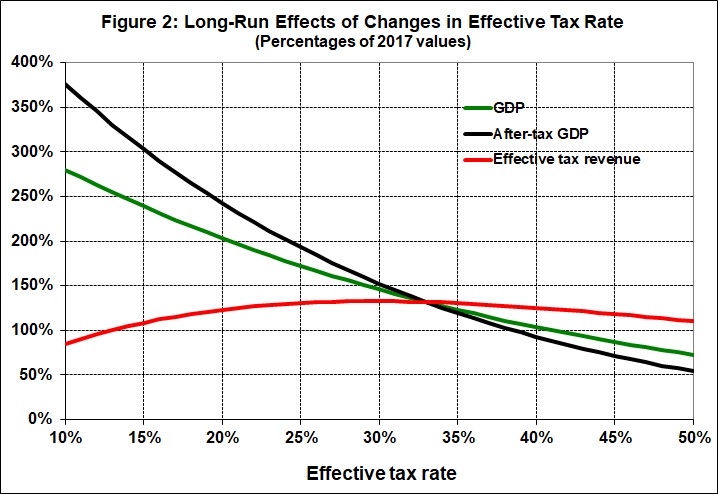
Note that the same real tax revenue would be realized at an effective tax rate of 13 percent of GDP. At that rate, GDP would rise to 2.5 times its 2017 value (instead of 1.6 times as shown in Figure 1), and after-tax GDP would rise to 3.3 times its 2017 value (instead of 2.1 times as shown in Figure 1).

The real Laffer curve — the one that people ought to pay attention to — is the Rahn curve. Holding everything else constant, here is the relationship between the real growth rate and the effective tax rate:

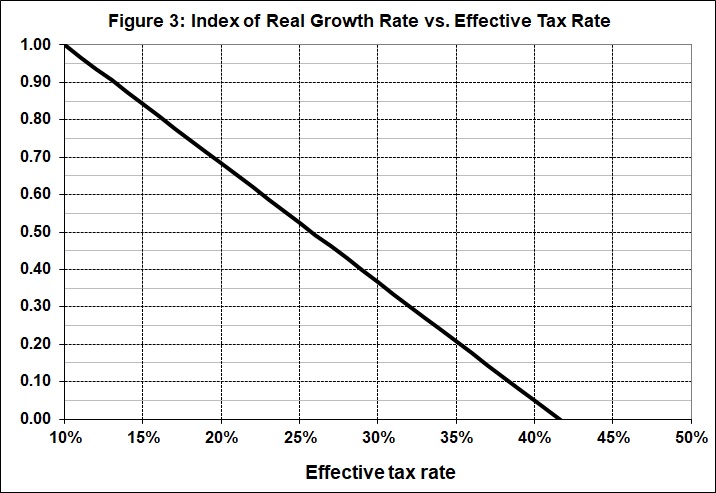
At the current effective tax rate — 33 percent of GDP — the economy is limping along at about one-third of its potential growth. That is actually good news, inasmuch as the real growth rate dipped perilously close to 1 percent several times during the Obama administration, even after the official end of the Great Recession.

But it will take many years of spending cuts (relative to GDP, at least) and deregulation to push growth back to where it was in the decades immediately after World War II. Five percent isn’t out of the question.
__________

1. Total government spending, when transfer payments were negligible, amounted to between 5 and 10 percent of GDP between the Civil War and the Great Depression (Series F216-225, “Percent Distribution of National Income or Aggregate Payments, by Industry, in Current Prices: 1869-1968,” in Chapter F, National Income and Wealth, Historical Statistics of the United States, Colonial Times to 1970: Part 1). The cost of an adequate defense is a lot higher than it was in those relatively innocent times. Defense spending now accounts for about 3.5 percent of GDP. An increase to 5 percent wouldn’t render the U.S. invulnerable, but it would do a lot to deter potential adversaries. So at 10 percent of GDP, government spending on policing, the administration of justice, and defense — and nothing else — should be more than adequate to sustain the rule of law.

2. The effective tax rate on GDP in 2017 was 33.4 percent. That number represents total government government expenditures (line 37 of BEA Table 3.1), divided GDP (line 1 of BEA Table 1.15). The nominal tax rate on GDP was 30 percent; that is, government receipts (line 34 of BEA Table 3.1) accounted for 30 percent of GDP. (The BEA tables are accessible here.) I use the effective tax rate in this analysis because it truly represents the direct costs levied on the economy by government. (The indirect cost of regulatory activity adds about $2 trillion, bringing the total effective tax to 44 percent.)