You may not know about the Rahn Curve, but it’s central to the story I’m about to tell. The theory behind the Rahn Curve is simple — but not simplistic. A relatively small government with powers limited mainly to the protection of citizens and their property is worth more than its cost to taxpayers because it fosters productive economic activity (not to mention liberty). But additional government spending hinders productive activity in many ways, which are discussed in Daniel Mitchell’s paper, “The Impact of Government Spending on Economic Growth.” (I would add to Mitchell’s list the burden of regulatory activity, which grows even when government does not.)
What does the Rahn Curve look like? Mitchell estimates this relationship between government spending and economic growth:

The curve is dashed rather than solid at low values of government spending because it has been decades since the governments of developed nations have spent as little as 20 percent of GDP. But as Mitchell and others note, the combined spending of governments in the U.S. was 10 percent (and less) until the eve of the Great Depression. And it was in the low-spending, laissez-faire era from the end of the Civil War to the early 1900s that the U.S. enjoyed its highest sustained rate of economic growth.
Elsewhere, I estimated the Rahn curve that spans most of the history of the United States. I came up with this relationship (terms modified for simplicity (with a slight cosmetic change in terminology):
Yg = 0.054 -0.066F
To be precise, it’s the annualized rate of growth over the most recent 10-year span (Yg), as a function of F (fraction of GDP spent by governments at all levels) in the preceding 10 years. The relationship is lagged because it takes time for government spending (and related regulatory activities) to wreak their counterproductive effects on economic activity. Also, I include transfer payments (e.g., Social Security) in my measure of F because there’s no essential difference between transfer payments and many other kinds of government spending. They all take money from those who produce and give it to those who don’t (e.g., government employees engaged in paper-shuffling, destructive social-engineering schemes, and counterproductive regulatory activities).
When F is greater than the amount needed for national defense and domestic justice — no more than 0.1 (10 percent of GDP) — it discourages productive, growth-producing, job-creating activity. And because government spending weighs most heavily on taxpayers with above-average incomes, higher rates of F also discourage saving, which finances growth-producing investments in new businesses, business expansion, and capital (i.e., new and more productive business assets, both physical and intellectual).
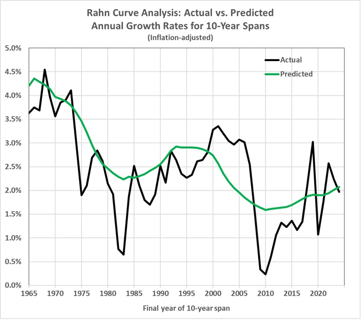
I’ve taken a closer look at the post-World War II numbers because of the marked decline in the real rate of GDP growth since the end of the war. (A smoothed trend drops from 4.3 percent in 1947 to 1.5 percent in 2024.)
Here’s the revised result, which spans 1946-2024 and accounts for more variables:
Yg = -0.0417lnF + 0.105lnA – 0.0104lnR
Where,
Yg = real rate of GDP growth in a 10-year span (annualized)
lnF = natural logarithm of the fraction of GDP spent by governments at all levels during the preceding 10 years
lnA = natural logarithm of the constant-dollar value of private nonresidential assets (business assets) as a fraction of GDP, averaged over the preceding 10 years
lnR = natural logarithm of the average number of Federal Register pages, in thousands, for the preceding 10-year period
(The r-squared of the equation is 0.97 and the F-value is 5.03E-44. The p-values of the coefficients are 4.16E-28, 6.59E-10, and 2.3E-14. The standard error of the estimate is 0.0046, that is, about one-half of a percentage point.)
Here’s how the equation stacks up against actual 10-year rates of real GDP growth:
What does the equation portend for the next 10 years? Based on the most recent values of F, A, and R, the real rate of growth for the next 10 years will be 1.6 to 2.6 percent. That would be reduction from the year-over-year rate for the fourth quarter of 2024, which was 2.5 percent, and about the same as the 10-year average for 2015-2024, which was 2.1 percent.
The coefficients yield some insights into the effects of policy changes.
- A reduction of F by 5 percentage points would raise the rate of growth by 0.6 percentage point, which is a big boost considering the current rate of growth.
- If A were to rise by 10 percentage points (that is, to the level of the early 1980s), the rate of growth would rise by 0.8 percentage point — another big boost.
- If R were to be cut from 107 (the 2024 value) to 90 (the 2023 value), the rate of growth would rise by 0.2 percentage point — nothing to sneeze at.
The cumulative effect of the preceding changes would cause the rate of growth to rise by 1.6 percentage points. The resulting increase to a growth rate of about 4 percent would be a big deal. At a real rate of 2 percent, the economy doubles every 36 years; at a real rate of 4 percent, there’s a doubling every 18 years.
To look at it another way: If GDP grows at the same rate as population (i.e., about 2 percent), there’s no growth in per-capita GDP. Everything above 2 percent means a real rise per-capita GDP. The bonus is that a greater share of GDP would be produced by and for workers in the private sector.
