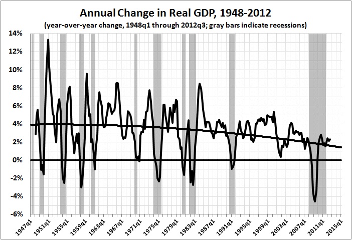
From “Keynesian Multiplier: Fiction vs. Fact“:

There are a few economic concepts that are widely cited (if not understood) by non-economists. Certainly, the “law” of supply and demand is one of them. The Keynesian (fiscal) multiplier is another; it is

the ratio of a change in national income to the change in government spending that causes it. More generally, the exogenous spending multiplier is the ratio of a change in national income to any autonomous change in spending (private investment spending, consumer spending, government spending, or spending by foreigners on the country’s exports) that causes it.

The multiplier is usually invoked by pundits and politicians who are anxious to boost government spending as a “cure” for economic downturns. What’s wrong with that? If government spends an extra $1 to employ previously unemployed resources, why won’t that $1 multiply and become $1.50, $1.60, or even $5 worth of additional output?

What’s wrong is the phony math by which the multiplier is derived, and the phony story that was long ago concocted to explain the operation of the multiplier….

To show why the math is phony, I’ll start with a derivation of the multiplier. The derivation begins with the accounting identity Y = C + I + G, which means that total output (Y) = consumption (C) + investment (I) + government spending (G)….

Now, let’s say that b = 0.8. This means that income-earners, on average, will spend 80 percent of their additional income on consumption goods (C), while holding back (saving, S) 20 percent of their additional income. With b = 0.8, k = 1/(1 – 0.8) = 1/0.2 = 5. That is, every $1 of additional spending — let us say additional government spending (∆G) rather than investment spending (∆I) — will yield ∆Y = $5. In short, ∆Y = k(∆G), as a theoretical maximum.

But:

[The multiplier] it isn’t a functional representation — a model — of the dynamics of the economy. Assigning a value to b (the marginal propensity to consume) — even if it’s an empirical value — doesn’t alter that fact that the derivation is nothing more than the manipulation of a non-functional relationship, that is, an accounting identity.

Consider, for example, the equation for converting temperature Celsius (C) to temperature Fahrenheit (F): F = 32 + 1.8C. It follows that an increase of 10 degrees C implies an increase of 18 degrees F. This could be expressed as ∆F/∆C = k* , where k* represents the “Celsius multiplier”. There is no mathematical difference between the derivation of the investment/government-spending multiplier (k) and the derivation of the Celsius multiplier (k*). And yet we know that the Celsius multiplier is nothing more than a tautology; it tells us nothing about how the temperature rises by 10 degrees C or 18 degrees F. It simply tells us that when the temperature rises by 10 degrees C, the equivalent rise in temperature F is 18 degrees. The rise of 10 degrees C doesn’t cause the rise of 18 degrees F.

Therefore:

[T]he Keynesian investment/government-spending multiplier simply tells us that if ∆Y = $5 trillion, and if b = 0.8, then it is a matter of mathematical necessity that ∆C = $4 trillion and ∆I + ∆G = $1 trillion. In other words, a rise in I + G of $1 trillion doesn’t cause a rise in Y of $5 trillion; rather, Y must rise by $5 trillion for C to rise by $4 trillion and I + G to rise by $1 trillion. If there’s a causal relationship between ∆G and ∆Y, the multiplier doesn’t portray it.

In sum, the fiscal multiplier puts the cart before the horse. It begins with a non-functional, mathematical relationship, stipulates a hypothetical increase in GDP, and computes that increase in consumption (and other things) that would occur if that increase were to be realized.

As economist Steve Landsburg explains in “The Landsburg Multiplier: How to Make Everyone Rich”,

Murray Rothbard … observed that the really neat thing about this [fiscal stimulus] argument is that you can do exactly the same thing with any accounting identity. Let’s start with this one:

Y = L + E

Here Y is economy-wide income, L is Landsburg’s income, and E is everyone else’s income. No disputing that one.

Next we observe that everyone else’s share of the income tends to be about 99.999999% of the total. In symbols, we have:

E = .99999999 Y

Combine these two equations, do your algebra, and voila:

Y = 100,000,000

That 100,000,000 there is the soon-to-be-famous “Landsburg multiplier”. Our equation proves that if you send Landsburg a dollar, you’ll generate $100,000,000 worth of income for everyone else.

Send me your dollars, yearning to be free.

Tax cuts may stimulate economic activity, but not nearly to the extent suggested by the multiplier. Moreover, if government spending isn’t reduced at the same time that taxes are cut, and if there is something close to full employment of labor and capital, the main result of a tax cut will be inflation.

Government spending (as shown in “Keynsian Multiplier: Fact vs. Fiction” and “Economic Growth Since World War II“) doesn’t stimulate the economy, and usually has the effect of reducing private consumption and investment. That may be to the liking of big-government worshipers, but it’s bad for most of us.