Nassim Nicholas Taleb, in his best-selling Fooled by Randomness, charges human beings with the commission of many perceptual and logical errors. One reviewer captures the point of the book, which is to
explore luck “disguised and perceived as non-luck (that is, skills).” So many of the successful among us, he argues, are successful due to luck rather than reason. This is true in areas beyond business (e.g. Science, Politics), though it is more obvious in business.
Our inability to recognize the randomness and luck that had to do with making successful people successful is a direct result of our search for pattern. Taleb points to the importance of symbolism in our lives as an example of our unwillingness to accept randomness. We cling to biographies of great people in order to learn how to achieve greatness, and we relentlessly interpret the past in hopes of shaping our future.
Only recently has science produced probability theory, which helps embrace randomness. Though the use of probability theory in practice is almost nonexistent.
Taleb says the confusion between luck and skill is our inability to think critically. We enjoy presenting conjectures as truth and are not equipped to handle probabilities, so we attribute our success to skill rather than luck.
Taleb writes in a style found all too often on best-seller lists: pseudo-academic theorizing “supported” by selective (often anecdotal) evidence. I sometimes enjoy such writing, but only for its entertainment value. Fooled by Randomness leaves me unfooled, for several reasons.
THE FUNDAMENTAL FLAW
The first reason that I am unfooled by Fooled… might be called a meta-reason. Standing back from the book, I am able to perceive its essential defect: According to Taleb, human affairs — especially economic affairs, and particularly the operations of financial markets — are dominated by randomness. But if that is so, only a delusional person can truly claim to understand the conduct of human affairs. Taleb claims to understand the conduct of human affairs. Taleb is therefore either delusional or omniscient.
Given Taleb’s humanity, it is more likely that he is delusional — or simply fooled, but not by randomness. He is fooled because he proceeds from the assumption of randomness instead of exploring the ways and means by which humans are actually capable of shaping events. Taleb gives no more than scant attention to those traits which, in combination, set humans apart from other animals: self-awareness, empathy, forward thinking, imagination, abstraction, intentionality, adaptability, complex communication skills, and sheer brain power. Given those traits (in combination) the world of human affairs cannot be random. Yes, human plans can fail of realization for many reasons, including those attributable to human flaws (conflict, imperfect knowledge, the triumph of hope over experience, etc.). But the failure of human plans is due to those flaws — not to the randomness of human behavior.
What Taleb sees as randomness is something else entirely. The trajectory of human affairs often is unpredictable, but it is not random. For it is possible to find patterns in the conduct of human affairs, as Taleb admits (implicitly) when he discusses such phenomena as survivorship bias, skewness, anchoring, and regression to the mean.
A DISCOURSE ON RANDOMNESS
What Is It?
Taleb, having bloviated for dozens of pages about the failure of humans to recognize randomness, finally gets around to (sort of) defining randomness on pages 168 and 169 (of the 2005 paperback edition):
…Professor Karl Pearson … devised the first test of nonrandomness (it was in reality a test of deviation from normality, which for all intents and purposes, was the same thing). He examined millions of runs of [a roulette wheel] during the month of July 1902. He discovered that, with high degree of statistical significance … the runs were not purely random…. Philosophers of statistics call this the reference case problem to explain that there is no true attainable randomness in practice, only in theory….
…Even the fathers of statistical science forgot that a random series of runs need not exhibit a pattern to look random…. A single random run is bound to exhibit some pattern — if one looks hard enough…. [R]eal randomness does not look random.
The quoted passage illustrates nicely the superficiality of Fooled by Randomness, and (I must assume) the muddledness of Taleb’s thinking:
- He accepts a definition of randomness which describes the observation of outcomes of mechanical processes (e.g., the turning of a roulette wheel, the throwing of dice) that are designed to yield random outcomes. That is, randomness of the kind cited by Taleb is in fact the result of human intentions.
- If “there is no true attainable randomness,” why has Taleb written a 200-plus page book about randomness?
- What can he mean when he says “a random series of runs need not exhibit a pattern to look random”? The only sensible interpretation of that bit of nonsense would be this: It is possible for a random series of runs to contain what looks like a pattern. But remember that the random series of runs to which Taleb refers is random only because humans intended its randomness.
- It is true enough that “A single random run is bound to exhibit some pattern — if one looks hard enough.” Sure it will. But it remains a single random run of a process that is intended to produce randomness, which is utterly unlike such events as transactions in financial markets.
One of the “fathers of statistical science” mentioned by Taleb (deep in the book’s appendix) is Richard von Mises, who in Probability Statistics and Truth defines randomness as follows:
First, the relative frequencies of the attributes [e.g. heads and tails] must possess limiting values [i.e., converge on 0.5, in the case of coin tosses]. Second, these limiting values must remain the same in all partial sequences which may be selected from the original one in an arbitrary way. Of course, only such partial sequences can be taken into consideration as can be extended indefinitely, in the same way as the original sequence itself. Examples of this kind are, for instance, the partial sequences formed by all odd members of the original sequence, or by all members for which the place number in the sequence is the square of an integer, or a prime number, or a number selected according to some other rule, whatever it may be. (pp. 24-25 of the 1981 Dover edition, which is based on the author’s 1951 edition)
Gregory J. Chaitin, writing in Scientific American (“Randomness and Mathematical Proof,” vol. 232, no. 5 (May 1975), pp. 47-52), offers this:
We are now able to describe more precisely the differences between the[se] two series of digits … :
01010101010101010101
01101100110111100010
The first could be specified to a computer by a very simple algorithm, such as “Print 01 ten times.” If the series were extended according to the same rule, the algorithm would have to be only slightly larger; it might be made to read, for example, “Print 01 a million times.” The number of bits in such an algorithm is a small fraction of the number of bits in the series it specifies, and as the series grows larger the size of the program increases at a much slower rate.
For the second series of digits there is no corresponding shortcut. The most economical way to express the series is to write it out in full, and the shortest algorithm for introducing the series into a computer would be “Print 01101100110111100010.” If the series were much larger (but still apparently patternless), the algorithm would have to be expanded to the corresponding size. This “incompressibility” is a property of all random numbers; indeed, we can proceed directly to define randomness in terms of incompressibility: A series of numbers is random if the smallest algorithm capable of specifying it to a computer has about the same number of bits of information as the series itself [emphasis added].
This is another way of saying that if you toss a balanced coin 1,000 times the only way to describe the outcome of the tosses is to list the 1,000 outcomes of those tosses. But, again, the thing that is random is the outcome of a process designed for randomness.
Taking Mises and Chaitin’s definitions together, we can define random events as events which are repeatable, convergent on a limiting value, and truly patternless over a large number of repetitions. Evolving economic events (e.g., stock-market trades, economic growth) are not alike (in the way that dice are, for example), they do not converge on limiting values, and they are not patternless, as I will show.
In short, Taleb fails to demonstrate that human affairs in general or financial markets in particular exhibit randomness, properly understood.
Randomness and the Physical World
Nor are we trapped in a random universe. Returning to Mises, I quote from the final chapter of Probability, Statistics and Truth:
We can only sketch here the consequences of these new concepts [e.g., quantum mechanics and Heisenberg’s principle of uncertainty] for our general scientific outlook. First of all, we have no cause to doubt the usefulness of the deterministic theories in large domains of physics. These theories, built on a solid body of experience, lead to results that are well confirmed by observation. By allowing us to predict future physical events, these physical theories have fundamentally changed the conditions of human life. The main part of modern technology, using this word in its broadest sense, is still based on the predictions of classical mechanics and physics. (p. 217)
Even now, almost 60 years on, the field of nanotechnology is beginning to hardness quantum mechanical effects in the service of a long list of useful purposes.
The physical world, in other words, is not dominated by randomness, even though its underlying structures must be described probabilistically rather than deterministically.
Summation and Preview
A bit of unpredictability (or “luck”) here and there does not make for a random universe, random lives, or random markets. If a bit of unpredictability here and there dominated our actions, we wouldn’t be here to talk about randomness — and Taleb wouldn’t have been able to marshal his thoughts into a published, marketed, and well-sold book.
Human beings are not “designed” for randomness. Human endeavors can yield unpredictable results, but those results do not arise from random processes, they derive from skill or the lack therof, knowledge or the lack thereof (including the kinds of self-delusions about which Taleb writes), and conflicting objectives.
An Illustration from Life
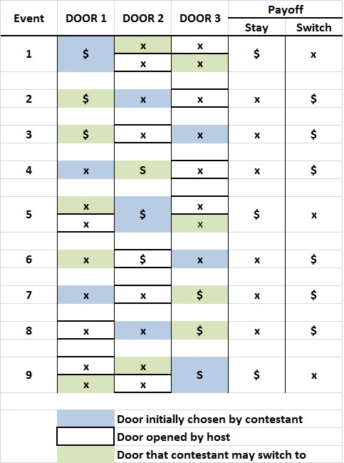
To illustrate my position on randomness, I offer the following digression about the game of baseball.
At the professional level, the game’s poorest players seldom rise above the low minor leagues. But even those poorest players are paragons of excellence when compared with the vast majority of American males of about the same age. Did those poorest players get where they were because of luck? Perhaps some of them were in the right place at the right time, and so were signed to minor league contracts. But their luck runs out when they are called upon to perform in more than a few games. What about those players who weren’t in the right place at the right time, and so were overlooked in spite of skills that would have advanced them beyond the rookie leagues? I have no doubt that there have been many such players. But, in the main, professional baseball abounds with the lion’s share of skilled baseball players who are there because they intend to be there, and because baseball clubs intend for them to be there.
Now, most minor leaguers fail to advance to the major leagues, even for the proverbial “cup of coffee” (appearing in few games at the end of the major-league season, when teams are allowed to expand their rosters following the end of the minor-league season). Does “luck” prevent some minor leaguers from advancement to “the show” (the major leagues)? Of course. Does “luck” result in the advancement of some minor leaguers to “the show”? Of course. But “luck,” in this context, means injury, illness, a slump, a “hot” streak, and the other kinds of unpredictable events that ballplayers are subject to. Are the events random? Yes, in the sense that they are unpredictable, but I daresay that most baseball players do not succumb to bad luck or advance very for or for very long because of good luck. In fact, ballplayers who advance to the major leagues, and then stay there for more than a few seasons, do so because they possess (and apply) greater skill than their minor-league counterparts. And make no mistake, each player’s actions are so closely watched and so extensively quantified that it isn’t hard to tell when a player is ready to be replaced.
It is true that a player may experience “luck” for a while during a season, and sometimes for a whole season. But a player will not be consistently “lucky” for several seasons. The length of his career (barring illness, injury, or voluntary retirement), and his accomplishments during that career, will depend mainly on his inherent skills and his assiduousness in applying those skills.
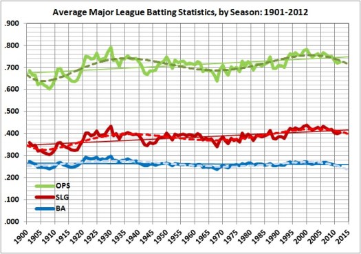
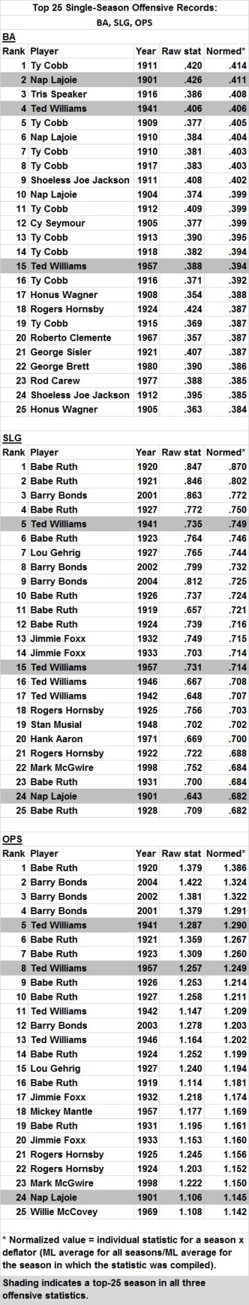
No one believes that Ty Cobb, Babe Ruth, Ted Williams, Christy Matthewson, Warren Spahn, and the dozens of other baseball players who rank among the truly great were lucky. No one believes that the vast majority of the the tens of thousands of minor leaguers who never enjoyed more than the proverbial cup of coffee were unlucky. No one believes that the vast majority of the millions of American males who never made it to the minor leagues were unlucky. Most of them never sought a career in baseball; those who did simply lacked the requisite skills.
In baseball, as in life, “luck” is mainly an excuse and rarely an explanation. We prefer to apply “luck” to outcomes when we don’t like the true explanations for them. In the realm of economic activity and financial markets, one such explanation (to which I will come) is the exogenous imposition of governmental power.
ARE ECONOMIC AND FINANCIAL OUTCOMES TRULY RANDOM?
They Cannot Be, Given Competition
Returning to Taleb’s main theme — the randomness of economic and financial events — I quote this key passage (my comments are in brackets and boldface):
…Most of [Bill] Gates'[s] rivals have an obsessive jealousy of his success. They are maddened by the fact that he managed to win so big while many of them are struggling to make their companies survive. [These are unsupported claims that I include only because they set the stage for what follows.]
Such ideas go against classical economic models, in which results either come from a precise reason (there is no account for uncertainty) or the good guy wins (the good guy is the one who is most skilled and has some technical superiority). [The “good guy” theory would come as a great surprise to “classical” economists, who quite well understood imperfect competition based on product differentiation and monopoly based on (among other things) early entry into a market.] Economists discovered path-dependent effects late in their game [There is no “late” in a “game” that had no distinct beginning and has no pre-ordained end.], then tried to publish wholesale on the topic that otherwise be bland and obvious. For instance, Brian Arthur, an economist concerned with nonlinearities at the Santa Fe Institute [What kinds of nonlinearities are found at the Santa Fe Institute?], wrote that chance events coupled with positive feedback other than technological superiority will determine economic superiority — not some abstrusely defined edge in a given area of expertise. [It would come as no surprise to economists — even “classical” ones — that many factors aside from technical superiority determine market outcomes.] While early economic models excluded randomness, Arthur explained how “unexpected orders, chance meetings with lawyers, managerial whims … would help determine which ones acheived early sales and, over time, which firms dominated.”
Regarding the final sentence of the quoted passage, I refer back to the example of baseball. A person or a firm may gain an opportunity to succeed because of the kinds of “luck” cited by Brian Arthur, but “good luck” cannot sustain an incompetent performer for very long. And when “bad luck” happens to competent individuals and firms they are often (perhaps usually) able to overcome it.
While overplaying the role of luck in human affairs, Taleb underplays the role of competition when he denigrates “classical economic models,” in which competition plays a central role. “Luck” cannot forever outrun competition, unless the game is rigged by governmental intervention, namely, the writing of regulations that tend to favor certain competitors (usually market incumbents) over others (usually would-be entrants). The propensity to regulate at the behest of incumbents (who plead “public interest,” of course) is a proof of the power of competition to shape economic outcomes. It is loathed and feared, and yet it leads us in the direction to which classical economic theory points: greater output and lower prices.
Competition is what ensures that (for the most part) the best ballplayers advance to the major leagues. It’s what keeps “monopolists” like Microsoft hopping (unless they have a government-guaranteed monopoly), because even a monopolist (or oligopolist) can face competition, and eventually lose to it — witness the former “Big Three” auto makers, many formerly thriving chain stores (from Kresge’s to Montgomery Ward’s), and numerous other brand names of days gone by. If Microsoft survives and thrives, it will be because it actually offers consumers more value for their money, either in the way of products similar to those marketed by Microsoft or in entirely new products that supplant those offered by Microsoft.
Monopolists and oligopolists cannot survive without constant innovation and attention to their customers’ needs.Why? Because they must compete with the offerors of all the other goods and services upon which consumers might spend their money. There is nothing — not even water — which cannot be produced or delivered in competitive ways. (For more, see this.)
The names of the particular firms that survive the competitive struggle may be unpredictable, but what is predictable is the tendency of competitive forces toward economic efficiency. In other words, the specific outcomes of economic competition may be unpredictable (which is not a bad thing), but the general result — efficiency — is neither unpredictable nor a manifestation of randomness or “luck.”
Taleb, had he broached the subject of competition would (with his hero George Soros) denigrate it, on the ground that there is no such thing as perfect competition. But the failure of competitive forces to mimic the model of perfect competition does not negate the power of competition, as I have summarized it here. Indeed, the failure of competitive forces to mimic the model of perfect competition is not a failure, for perfect competition is unattainable in practice, and to hold it up as a measure of the effectiveness of market forces is to indulge in the Nirvana fallacy.
In any event, Taleb’s myopia with respect to competition is so complete that he fails to mention it, let alone address its beneficial effects (even when it is less than perfect). And yet Taleb dares to dismiss as a utopist Milton Friedman (p. 272) — the same Milton Friedman who was among the twentieth century’s foremost advocates of the benefits of competition.
Are Financial Markets Random?
Given what I have said thus far, I find it almost incredible that anyone believes in the randomness of financial markets. It is unclear where Taleb stands on the random-walk hypothesis, but it is clear that he believes financial markets to be driven by randomness. Yet, contradictorily, he seems to attack the efficient-markets hypothesis (see pp. 61-62), which is the foundation of the random-walk hypothesis.
What is the random-walk hypothesis? In brief, it is this: Financial markets are so efficient that they instantaneously reflect all information bearing on the prices of financial instruments that is then available to persons buying and selling those instruments. (The qualifier “then available to persons buying and selling those instruments” leaves the door open for [a] insider trading and [b] arbitrage, due to imperfect knowledge on the part of some buyers and/or sellers.) Because information can change rapidly and in unpredictable ways, the prices of financial instruments move randomly. But the random movement is of a very special kind:
If a stock goes up one day, no stock market participant can accurately predict that it will rise again the next. Just as a basketball player with the “hot hand” can miss the next shot, the stock that seems to be on the rise can fall at any time, making it completely random.
And, therefore, changes in stock prices cannot be predicted.
Note, however, the focus on changes. It is that focus which creates the illusion of randomness and unpredictability. It is like hoping to understand the movements of the planets around the sun by looking at the random movements of a particle in a cloud chamber.
When we step back from day-to-day price changes, we are able to see the underlying reality: prices (instead of changes) and price trends (which are the opposite of randomness). This (correct) perspective enables us to see that stock prices (on the whole) are not random, and to identify the factors that influence the broad movements of the stock market.
For one thing, if you look at stock prices correctly, you can see that they vary cyclically. Here is a telling graphic (from “Efficient-market hypothesis” at Wikipedia):
 Price-Earnings ratios as a predictor of twenty-year returns based upon the plot by Robert Shiller (Figure 10.1,[18] source). The horizontal axis shows the real price-earnings ratio of the S&P Composite Stock Price Index as computed in Irrational Exuberance (inflation adjusted price divided by the prior ten-year mean of inflation-adjusted earnings). The vertical axis shows the geometric average real annual return on investing in the S&P Composite Stock Price Index, reinvesting dividends, and selling twenty years later. Data from different twenty-year periods is color-coded as shown in the key. See also ten-year returns. Shiller states that this plot “confirms that long-term investors—investors who commit their money to an investment for ten full years—did do well when prices were low relative to earnings at the beginning of the ten years. Long-term investors would be well advised, individually, to lower their exposure to the stock market when it is high, as it has been recently, and get into the market when it is low.”[18] This correlation between price to earnings ratios and long-term returns is not explained by the efficient-market hypothesis.
Why should stock prices tend to vary cyclically? Because stock prices generally are driven by economic growth (i.e., changes in GDP), and economic growth is strongly cyclical. (See this post.)
More fundamentally, the economic outcomes reflected in stock prices aren’t random, for they depend mainly on intentional behavior along well-rehearsed lines (i.e., the production and consumption of goods and services in ways that evolve over time). Variations in economic behavior, even when they are unpredictable, have explanations; for example:
- Innovation and capital investment spur the growth of economic output.
- Natural disasters slow the growth of economic output (at least temporarily) because they absorb resources that could have gone to investment (as well as consumption).
- Governmental interventions (taxation and regulation), if not reversed, dampen growth permanently.
There is nothing in those three statements that hasn’t been understood since the days of Adam Smith. Regarding the third statement, the general slowing of America’s economic growth since the advent of the Progressive Era around 1900 is certainly not due to randomness, it is due to the ever-increasing burden of taxation and regulation imposed on the economy — an entirely predictable result, and certainly not a random one.
In fact, the long-term trend of the stock market (as measured by the S&P 500) is strongly correlated with GDP. And broad swings around that trend can be traced to governmental intervention in the economy. The following graph shows how the S&P 500, reconstructed to 1870, parallel constant-dollar GDP:
The next graph shows the relationship more clearly.


The wild swings around the trend line began in the uncertain aftermath of World War I, which saw the imposition of production and price controls. The swings continued with the onset of the Great Depression (which can be traced to governmental action), the advent of the anti-business New Deal, and the imposition of production and price controls on a grand scale during World War II. The next downswing was occasioned by the culmination the Great Society, the “oil shocks” of the early 1970s, and the raging inflation that was touched off by — you guessed it — government policy. The latest downswing is owed mainly to the financial crisis born of yet more government policy: loose money and easy loans to low-income borrowers.
And so it goes, wildly but predictably enough if you have the faintest sense of history. The moral of the story: Keep your eye on government and a hand on your wallet.
CONCLUSION
There is randomness in economic affairs, but they are not dominated by randomness. They are dominated by intentions, including especially the intentions of the politicians and bureaucrats who run governments. Yet, Taleb has no space in his book for the influence of their deeds economic activity and financial markets.
Taleb is right to disparage those traders (professional and amateur) who are lucky enough to catch upswings, but are unprepared for downswings. And he is right to scoff at their readiness to believe that the current upswing (uniquely) will not be followed by a downswing (“this time it’s different”).
But Taleb is wrong to suggest that traders are fooled by randomness. They are fooled to some extent by false hope, but more profoundly by their inablity to perceive the economic damage wrought by government. They are not alone of course; most of the rest of humanity shares their perceptual failings.
Taleb, in that respect, is only somewhat different than most of the rest of humanity. He is not fooled by false hope, but he is fooled by non-randomness — the non-randomness of government’s decisive influence on economic activity and financial markets. In overlooking that influence he overlooks the single most powerful explanation for the behavior of markets in the past 90 years.


