Election 2020: A Penultimate Prognostication

Tomorrow I will issue a firm prediction about the outcome of the presidential election of 2020. I will base the prediction on the indicators discussed below.

The mood of the electorate was rising sharply in 2012 when Obama was re-elected. Recently, the mood has risen sharply from its COVID-induced depths, which is a good sign for Trump:

Trump’s standing with likely voters has, as measured by Rasmussen Reports, has rebounded to levels well above those attained by Obama at the same point in 2012:

According to White House Watch at Rasmussen Reports, which nailed Clinton’s popular-vote edge four years ago, Biden is not out-performing Clinton:

Biden’s narrow lead and Trump’s standing with likely voters translates into a slight edge in the electoral vote:

If I were calling the election today, I would call it for Trump — subject to the caveat that the outcomes in some key States may well hinge on decisions rendered by Democrat-appointed judges.

“It’s Tough to Make Predictions, Especially about the Future”

A lot of people have said it, or something like it, though probably not Yogi Berra, to whom it’s often attributed.

Here’s another saying, which is also apt here: History does not repeat itself. The historians repeat one another.

I am accordingly amused by something called cliodynamics, which is discussed at length by Amanda Rees in “Are There Laws of History?” (Aeon, May 2020). The Wikipedia article about cliodynamics describes it as

a transdisciplinary area of research integrating cultural evolution, economic history/cliometrics, macrosociology, the mathematical modeling of historical processes during the longue durée [the long term], and the construction and analysis of historical databases. Cliodynamics treats history as science. Its practitioners develop theories that explain such dynamical processes as the rise and fall of empires, population booms and busts, spread and disappearance of religions. These theories are translated into mathematical models. Finally, model predictions are tested against data. Thus, building and analyzing massive databases of historical and archaeological information is one of the most important goals of cliodynamics.

I won’t dwell on the methods of cliodynamics, which involve making up numbers about various kinds of phenomena and then making up models which purport to describe, mathematically, the interactions among the phenomena. Underlying it all is the practitioner’s broad knowledge of historical events, which he converts (with the proper selection of numerical values and mathematical relationships) into such things as the Kondratiev wave, a post-hoc explanation of a series of arbitrarily denominated and subjectively measured economic eras.

In sum, if you seek patterns you will find them, but pattern-making (modeling) is not science. (There’s a lot more here.)

Here’s a simple demonstration of what’s going on with cliodynamics. Using the RANDBETWEEN function of Excel, I generated two columns of random numbers ranging in value from 0 to 1,000, with 1,000 numbers in each column. I designated the values in the left column as x variables and the numbers in the right column as y variables. I then arbitrarily chose the first 10 pairs of numbers and plotted them:

As it turns out, the relationship, even though it seems rather loose, has only a 21-percent chance of being due to chance. In the language of statistics, two-tailed p=0.21.

Of course, the relationship is due entirely to chance because it’s the relationship between two sets of random numbers. So much for statistical tests of “significance”.

Moreover, I could have found “more significant” relationships had I combed carefully through the 1,000 pairs of random number with my pattern-seeking brain.

But being an honest person with scientific integrity, I will show you the plot of all 1,000 pairs of random numbers:

I didn’t bother to find a correlation between the x and y values because there is none. And that’s the messy reality of human history. Yes, there have been many determined (i.e., sought-for) outcomes  — such as America’s independence from Great Britain and Hitler’s rise to power. But they are not predetermined outcomes. Their realization depended on the surrounding circumstances of the moment, which were myriad, non-quantifiable, and largely random in relation to the event under examination (the revolution, the putsch, etc.). The outcomes only seem inevitable and predictable in hindsight.

Cliodynamics is a variant of the anthropic principle, which is that he laws of physics appear to be fine-tuned to support human life because we humans happen to be here to observe the laws of physics. In the case of cliodynamics, the past seems to consist of inevitable events because we are here in the present looking back (rather hazily) at the events that occurred in the past.

Cliodynametricians, meet Nostradamus. He “foresaw” the future long before you did.

Predicting “Global” Temperatures — An Analogy with Baseball

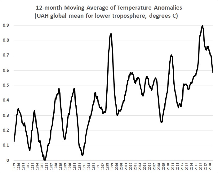
The following graph is a plot of the 12-month moving average of “global” mean temperature anomalies for 1979-2018 in the lower troposphere, as reported by the climate-research unit of the University of Alabama-Huntsville (UAH):

The UAH values, which are derived from satellite-borne sensors, are as close as one can come to an estimate of changes in “global” mean temperatures. The UAH values certainly are more complete and reliable than the values derived from the surface-thermometer record, which is biased toward observations over the land masses of the Northern Hemisphere (the U.S., in particular) — observations that are themselves notoriously fraught with siting problems, urban-heat-island biases, and “adjustments” that have been made to “homogenize” temperature data, that is, to make it agree with the warming predictions of global-climate models.

The next graph roughly resembles the first one, but it’s easier to describe. It represents the fraction of games won by the Oakland Athletics baseball team in the 1979-2018 seasons:

Unlike the “global” temperature record, the A’s W-L record is known with certainty. Every game played by the team (indeed, by all teams in organized baseball) is diligently recorded, and in great detail. Those records yield a wealth of information not only about team records, but also about the accomplishments of the individual players whose combined performance determines whether and how often a team wins its games. Given that information, and much else about which statistics are or could be compiled (records of players in the years and games preceding a season or game; records of each team’s owner, general managers, and managers; orientations of the ballparks in which each team compiled its records; distances to the fences in those ballparks; time of day at which games were played; ambient temperatures, and on and on).

Despite all of that knowledge, there is much uncertainty about how to model the interactions among the quantifiable elements of the game, and how to give weight to the non-quantifiable elements (a manager’s leadership and tactical skills, team spirit, and on and on). Even the professional prognosticators at FiveThirtyEight, armed with a vast compilation of baseball statistics from which they have devised a complex predictive model of baseball outcomes will admit that perfection (or anything close to it) eludes them. Like many other statisticians, they fall back on the excuse that “chance” or “luck” intrudes too often to allow their statistical methods to work their magic. What they won’t admit to themselves is that the results of simulations (such as those employed in the complex model devised by FiveThirtyEight),

reflect the assumptions underlying the authors’ model — not reality. A key assumption is that the model … accounts for all relevant variables….

As I have said, “luck” is mainly an excuse and rarely an explanation. Attributing outcomes to “luck” is an easy way of belittling success when it accrues to a rival.

It is also an easy way of dodging the fact that no model can accurately account for the outcomes of complex systems. “Luck” is the disappointed modeler’s excuse.

If the outcomes of baseball games and seasons could be modeled with great certainly, people wouldn’t bet on those outcomes. The existence of successful models would become general knowledge, and betting would cease, as the small gains that might accrue from betting on narrow odds would be wiped out by vigorish.

Returning now to “global” temperatures, I am unaware of any model that actually tries to account for the myriad factors that influence climate. The pseudo-science of “climate change” began with the assumption that “global” temperatures are driven by human activity, namely the burning of fossil fuels that releases CO2 into the atmosphere. CO2 became the centerpiece of global climate models (GCMs), and everything else became an afterthought, or a non-thought. It is widely acknowledged that cloud formation and cloud cover — obviously important determinants of near-surface temperatures — are treated inadequately (when treated at all). The mechanism by which the oceans absorb heat and transmit it to the atmosphere also remain mysterious. The effect of solar activity on cosmic radiation reaching Earth (and thus on cloud formation) remains is often dismissed despite strong evidence of its importance. Other factors that seem to have little or no weight in GCMs (though they are sometimes estimated in isolation) include plate techtonics, magma flows, volcanic activity, and vegetation.

Despite all of that, builders of GCMs — and the doomsayers who worship them — believe that “global” temperatures will rise to catastrophic readings. The rising oceans will swamp coastal cities; the earth will be scorched. except where it is flooded by massive storms; crops will fail accordingly; tempers will flare and wars will break out more frequently.

There’s just one catch, and it’s a big one. Minute changes in the value of a dependent variable (“global” temperature, in this case) can’t be explained by a model in which key explanatory variables are unaccounted for, about which there is much uncertainty surrounding the values of those explanatory variables that can be accounted for, and about which there is great uncertainty about the mechanisms by which the variables interact. Even an impossibly complete model would be wildly inaccurate given the uncertainty of the interactions among variables and the values of those variables (in the past as well as in the future).

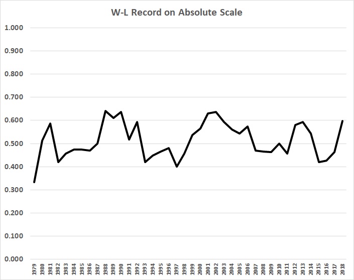
I say “minute changes” because first graph above is grossly misleading. An unbiased depiction of “global” temperatures looks like this:

There’s a much better chance of predicting the success or failure of the Oakland A’s, whose record looks like this on an absolute scale:

Just as no rational (unemotional) person should believe that predictions of “global” temperatures should dictate government spending and regulatory policies, no sane bettor is holding his breath in anticipation that the success or failure of the A’s (or any team) can be predicted with bankable certainty.

All of this illustrates a concept known as causal density, which Arnold Kling explains:

When there are many factors that have an impact on a system, statistical analysis yields unreliable results. Computer simulations give you exquisitely precise unreliable results. Those who run such simulations and call what they do “science” are deceiving themselves.

The folks at FiveThirtyEight are no more (and no less) delusional than the creators of GCMs.

More Stock-Market Analysis (II)

Today’s trading on U.S. stock markets left the Wilshire 5000 Total Market Full-Cap index 17 percent below its September high. How low will the market go? When will it bounce back? There’s no way to know, which is the main message of “Shiller’s Folly” and “More Stock-Market Analysis“.

Herewith are three relevant exhibits based on the S&P Composite index as reconstructed by Robert Shiller (commentary follows):

In the following notes, price refers to the value of the index; real price is the inflation-adjusted value of the index; total return is the value with dividends reinvested; real total return is the inflation-adjusted value of total return.

  • The real price trend represents an annualized gain of 1.8 percent (through November 2018).
  • The real total return trend represents an annualized gain of 6.5 percent (through September 2018).
  • In month-to-month changes, real price has gone up 56 percent of the time; real total return has gone up 61 percent of the time.
  • Real price has been in a major decline about 24 percent of the time, where a major decline is defined as a real price drop of more than 25 percent over a span of at least 6 months.
  • The picture is a bit less bleak for total returns (about 20 percent of the time) because the reinvestment of dividends somewhat offsets price drops.
  • Holding a broad-market index fund is never a sure thing. Returns fluctuate wildly. Impressive real returns (e.g., 20 percent and higher) are possible in the shorter run (e.g., 5-10 years), but so are significantly negative returns. Holding a fund longer reduces the risk of a negative return while also suppressing potential gains.
  • Long-run real returns of greater than 5 percent a year are not to be scoffed at. It takes a lot of research, patience, and luck to do better than that with individual stocks and specialized mutual funds.

More Stock-Market Analysis

I ended “Shiller’s Folly” with the Danish proverb, it is difficult to make predictions, especially about the future.

Here’s more in that vein. Shiller uses a broad market index, the S&P Composite (S&P), which he has reconstructed back to January 1871. I keep a record of the Wilshire 5000 Full-Cap Total-Return Index (WLX), which dates back to December 1970. When dividends for stocks in the S&P index are reinvested, its performance since December 1970 is almost identical to that of the WLX:

It is a reasonable assumption that if the WLX extended back to January 1871 its track record would nearly match that of the S&P. Therefore, one might assume that past returns on the WLX are a good indicator of future returns. In fact, the relationship between successive 15-year periods is rather strong:

But that seemingly strong relationship is an artifact of the relative brevity of the track record of the WLX.  Compare the relationship in the preceding graph with the analogous one for the S&P, which goes back an additional 100 years:

The equations are almost identical — and they predict almost the same real returns for the next 15 years: about 6 percent a year. But the graph immediately above should temper one’s feeling of certainty about the long-run rate of return on a broad market index fund or a well-diversified portfolio of stocks.


Related posts:
Stocks for the Long Run?
Stocks for the Long Run? (Part II)
Bonds for the Long Run?
Much Ado about the Price-Earnings Ratio
Whither the Stock Market?
Shiller’s Folly

Shiller’s Folly

Robert Shiller‘s most famous (or infamous) book, is Irrational Exuberance (2000). According to the Wikipedia article about the book,

the text put forth several arguments demonstrating how the stock markets were overvalued at the time. The stock market collapse of 2000 happened the exact month of the book’s publication.

The second edition of Irrational Exuberance was published in 2005 and was updated to cover the housing bubble. Shiller wrote that the real estate bubble might soon burst, and he supported his claim by showing that median home prices were six to nine times greater than median income in some areas of the country. He also showed that home prices, when adjusted for inflation, have produced very modest returns of less than 1% per year. Housing prices peaked in 2006 and the housing bubble burst in 2007 and 2008, an event partially responsible for the Worldwide recession of 2008-2009.

However, as the Wikipedia article notes,

some economists … challenge the predictive power of Shiller’s publication. Eugene Fama, the Robert R. McCormick Distinguished Service Professor of Finance at The University of Chicago and co-recipient with Shiller of the 2013 Nobel Prize in Economics, has written that Shiller “has been consistently pessimistic about prices,”[ so given a long enough horizon, Shiller is bound to be able to claim that he has foreseen any given crisis.

(A stopped watch is right twice a day, but wrong 99.9 percent of the time if read to the nearest minute. I also predicted the collapse of 2000, but four years too soon.)

One of the tools used by Shiller is a cyclically-adjusted price-to-earnings ratio known as  CAPE-10 . It is

a valuation measure usually applied to the US S&P 500 equity market. It is defined as price divided by the average of ten [previous] years of earnings … , adjusted for inflation. As such, it is principally used to assess likely future returns from equities over timescales of 10 to 20 years, with higher than average CAPE values implying lower than average long-term annual average returns.

CAPE-10, like other economic indicators of which I know, is a crude tool:

For example, the annualized real rate of price growth for the S&P Composite Index from October 2003 to October 2018 was 4.6 percent. The value of CAPE-10 in October 2003 was 25.68. According to the equation in the graph (which includes the period from October 2003 through October 2018), the real rate of price growth should have been -0.6 percent. The actual rate is at the upper end of the wide range of uncertainty around the estimate.

Even a seemingly more robust relationship yields poor results. Consider this one:

The equation in this graph produces a slightly better but still terrible estimate: price growth of -0.2 percent over the 15 years ending in October 2018.

If you put stock (pun intended) in the kinds of relationships depicted above, you should expect real growth in the S&P Composite Index to be zero for the next 15 years — plus or minus about 6 percentage points. It’s the plus or minus that matters — a lot — and the equations don’t help you one bit.

As the Danish proverb says, it is difficult to make predictions, especially about the future.